REVIEW 3 major objections 8 minor 14 references
Network weights alone reveal phase transitions and scaling laws
Reviewed by Pith at T0; open to challenge. T0 means a machine referee read the full paper against a public rubric. the ladder, T0–T4 →
T0 review · glm-5.2
2026-07-09 19:25 UTC pith:OM7HE6KJ
load-bearing objection Solid novel framework with one overstated contribution; the FSS claim needs either validation or downgrading the 3 major comments →
Weight-Space Physics: Interpretable Hypernetworks for Lattice Quantum Field Theories
The pith
A machine-rendered reading of the paper's core claim, the machinery that carries it, and where it could break.
Core claim
When a JEPA-based weight generator is trained to map the coupling constants of 2D scalar lattice field theory to the parameters of normalizing flow samplers, the resulting latent space geometry recovers three pieces of physical structure without any supervision from observables: the correct intrinsic dimension of the coupling manifold (estimated at 2.01 ± 0.06), the location of the phase transition (via a pullback-metric ridge concentrated in the network's non-local weight groups), and a finite-size scaling organization across lattice sizes consistent with the Ising exponent ν ≈ 1. The same architecture also generates functional flow samplers at unseen couplings, outperforming reconstruction
What carries the argument
JEPAWG consists of four components: a weight encoder that maps a 19,689-dimensional flow parameter vector to a latent embedding; a coupling encoder that maps the two bare couplings (m², λ) to the same latent space; a predictor trained to align coupling embeddings with weight embeddings via a VICReg invariance-plus-variance objective (with the covariance term deliberately removed so the latent space can concentrate onto the physically relevant low dimensions); and a decoder that maps predicted latent vectors back to flow parameters. The pullback metric on the weight map θ(g) — specifically its area element √det G(g) computed via finite differences in coupling space — serves as the geometric工具
Load-bearing premise
The cross-lattice scaling result depends on the hypothesis that the JEPAWG encoder, trained only to align coupling and weight embeddings at a single lattice size, should also place physically similar theories (related by finite-size scaling) close together across different lattice sizes. Nothing in the training objective enforces this cross-lattice proximity, and the recovered exponents span a wide range (0.55–2.34) depending on how the critical line is estimated.
What would settle it
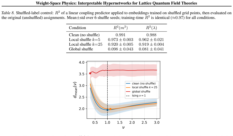
If the latent-space geometry were driven by coupling-space smoothness rather than physics, then shuffling the coupling-to-weight correspondence before training should destroy the phase-transition ridge and the finite-size scaling minimum. The authors perform this control (Appendix G): a global shuffle collapses coupling decodability (R² → 0.08) and eliminates the FSS minimum near ν = 1, while local shuffles preserve both. This confirms the physical structure is genuinely encoded in the weights, not an architectural artifact.
If this is right
- If network weights encode physical structure without explicit supervision, then trained neural samplers in lattice field theory can serve as diagnostic tools: one can probe for phase transitions and critical behavior by inspecting weight geometry rather than running expensive new simulations.
- The concentration of the phase-transition signal in non-local weight groups (zero-mode scaling and Fourier scaling) suggests a principled way to identify which parts of a neural network carry the physically relevant information, enabling targeted architecture design or pruning.
- The framework extends naturally to other quantum field theories with known phase structure, providing a falsifiable testbed for neural network interpretability research that lacks ground truth in standard ML settings.
- If the cross-lattice scaling result holds at larger lattice sizes, weight-space geometry could become a complementary method for estimating critical exponents, though the current precision (ν ranging 0.55–2.34 depending on estimator) is far from competitive with established methods.
Where Pith is reading between the lines
- The claim that weights function as a 'new type of physical observable' implies that different training procedures or architectures for the same physical theory should produce weight geometries with isomorphic physical structure — a testable prediction the paper does not make but which would strengthen the observable interpretation.
- If the latent space organizes by RG scaling variables without being told to, this suggests that the JEPA objective is implicitly biased toward discovering reparameterization-invariant structure — which would mean the approach might generalize to other systems with hidden symmetry or scaling structure beyond physics.
- The removal of the VICReg covariance term to preserve low-dimensional structure hints at a tension between standard representation-learning regularization (which spreads information across all latent dimensions) and physical interpretability (which requires the latent space to respect the actual dimensionality of the underlying manifold). This trade-off likely appears in other scientific ML applic
Editorial analysis
A structured set of objections, weighed in public.
Referee Report
Summary. This manuscript introduces JEPAWG, a Joint-Embedding Predictive Architecture (JEPA) that maps lattice field theory coupling constants to normalizing-flow weight parameters via a learned latent space. The work addresses two complementary questions: (1) as a diagnostic, does the geometry of trained flow weights recover physical structure (phase transitions, intrinsic dimensionality, finite-size scaling) without physics supervision, and (2) as a generator, can flow weights be predicted for unseen couplings? Applied to 2D phi^4 theory on lattices from 6^2 to 11^2, the authors report that the JEPAWG latent space recovers the correct intrinsic dimension (MLE 2.01±0.06), exhibits a pullback-metric ridge tracking the critical line in non-local weight groups, and encodes a finite-size scaling shift broadly consistent with the 2D Ising exponent nu=1. As a generator, JEPAWG outperforms PCA, AE, and VAE baselines on interpolation and extrapolation tasks, particularly in a multi-seed setting with weight-space discontinuities.
Significance. The paper's conceptual framing — treating lattice field theory as a testbed for neural network interpretability with known physical ground truth — is valuable and well-motivated. The intrinsic dimension recovery (Table 2) and the phase-transition ridge analysis (Figure 3, Table 3) are genuinely interesting results: the attribution of criticality signals to non-local parameter groups (theta_zero_mode, theta_scale) while bulk groups remain featureless is a non-trivial, physically interpretable finding. The weight canonicalization procedure (Appendix A.3) is a thoughtful treatment of weight-space symmetries. The multi-seed experimental design, which deliberately introduces weight-space discontinuities, strengthens the claim that JEPAWG learns physics rather than inheriting structure from a single conditional flow. The shuffled-label control (Appendix G) provides a useful falsifiability check on the coupling-encoding claim. The generator results (Table 1) demonstrate practical utility for amortizing flow training across couplings.
major comments (3)
- §5.4, §D.3, §B.1 — The cross-lattice FSS analysis applies the encoder of the larger lattice to zero-padded smaller-lattice weights without retraining (§D.3: 'the embeddings of both lattices are computed with the encoder of the larger lattice, applied to the smaller-lattice weights without retraining'). The smaller-lattice weights are zero-padded to match the larger lattice's parameter shape (§B.1: 'we align networks across lattice sizes to a common parameter shape by zero-padding smaller lattices and truncating larger ones in Fourier space'). This means the L=11 encoder processes input vectors with large blocks of artificial zeros it has never seen during training — a significant out-of-distribution application. The FSS minimum could arise from how the encoder maps zero-padded vectors (which have systematically different norm and structure) rather than from genuine RG structure in the权重.
- §5.4 — The cross-lattice proximity assumption ('if the latent geometry has captured the physics, weights that are FSS partners across different lattice sizes should lie nearer in embedding space than weights at unrelated couplings') is a hypothesis about what the encoder should do, not a consequence of the training objective. The VICReg invariance term (Eq. 7) enforces P(z_g) ≈ z_theta only within a single lattice size. Nothing in the loss enforces cross-lattice proximity under FSS scaling. The shuffled-label control (Appendix G) confirms the encoder extracts coupling information from weights, but it does not validate the cross-lattice proximity hypothesis. The authors should either provide additional evidence (e.g., training a cross-lattice JEPAWG on paired FSS partners) or more sharply delineate this as an unvalidated assumption. The scatter in nu* (0.55–2.34 across pairings and estim,
- §5.4, Table 5 — The recovered nu* values span 0.55 to 2.34 depending on the critical-line estimator and lattice pairing (Table 5). While the authors acknowledge this is a 'qualitative rather than precise match,' the claim in the abstract and contributions list that the latent geometry 'encodes a finite-size shift aligned with the 2D Ising exponent nu ≈ 1' is stronger than the data supports. The median over 15 pairings is 0.98 for the chi-peak estimator and 1.21 for the U4 crossing estimator, but individual pairings deviate substantially (e.g., 6→7 gives nu* = 2.34 for U4 crossing, 9→10 gives 0.55 for chi-peak). The abstract should be qualified to reflect the level of precision achieved, and the contributions list (item iii) should note the range rather than stating broad consistency without qualification.
minor comments (8)
- Table 1: The 'Raw Interp.' column conflates two different experimental conditions (raw weights, single-seed-like smooth manifold) with the canonicalized multi-seed results in the other columns. A footnote or separate panel clarifying that Raw Interp. uses uncanonicalized weights in the same multi-seed setting would help the reader.
- §4.1: The choice d_z = 16 is described as 'deliberately over-sizing the latent space relative to the two-dimensional coupling manifold.' It would be useful to report how sensitive the intrinsic dimension and generation results are to this choice (e.g., d_z = 4, 8, 32).
- §5.3, Table 3: The correlation between A_c(g) and chi for theta_scale is r = +0.51, which is positive but modest. The text describes this as exhibiting 'positive correlations' alongside theta_zero_mode (r = +0.67). The weaker correlation for theta_scale should be acknowledged more carefully.
- Figure 2: The AE panel shows PC1 capturing only 37.9% of variance, but the text states 51.0% for the leading two components. Showing the cumulative variance explained or the scree plot would aid comparison.
- §B.1: The statement 'we align networks across lattice sizes to a common parameter shape by zero-padding smaller lattices and truncating larger ones in Fourier space' needs more detail on how truncation affects the larger-lattice weights when embedded by the smaller-lattice encoder (if this direction is ever used).
- Appendix C, Table 4: The single-seed results show that PCA with an MLP head achieves 0.947 ESS on the interior, close to JEPAWG's 0.976. This suggests that in the smooth single-seed setting, the JEPAPA advantage is primarily in extrapolation. This nuance should be mentioned in the main text to strengthen the narrative.
- The term 'weight-space physics' is evocative but could be confused with physics-inspired optimization methods. A brief clarification in the introduction would help readers find this work.
- References: The citation to Cheng & Stratikopoulou (2026) and Gerdes & Cheng (2026) list future dates; please verify these are correct preprint dates.
Circularity Check
Intrinsic-dimension recovery is mildly self-consistent with the 2D coupling input; all other claims have independent content.
specific steps
-
self definitional
[Section 4.1 (Training) and contribution (i) in Section 1/Section 5.3]
"the JEPAWG latent space matches the 2D coupling manifold (MLE intrinsic dimension 2.01±0.06; 98.5% of variance in two principal axes)... we set dz = 16, deliberately over-sizing the latent space relative to the two-dimensional coupling manifold so that any concentration onto fewer dimensions is a learned property rather than an architectural constraint."
The coupling encoder Eg maps R^2 → R^{16}, and the VICReg invariance term (Eq. 7, weight α=25) directly penalizes ||P(zg) − zθ||², forcing the weight embedding zθ to lie near the image of P∘Eg, which is a function of a 2D input and thus has intrinsic dimension ≤ 2. The recovery of intrinsic dimension 2 is therefore largely a consequence of the training objective: the method is given 2D coupling input and the invariance loss forces the weight embedding to align with it. The variance term (β=25) provides some resistance by penalizing collapsed dimensions, but it only penalizes dimensions with std < 1, a weaker constraint than the direct L2 pull of the invariance term. The framing as 'a learned property rather than an architectural constraint' overstates the surprise: the 2D structure is not,
full rationale
The paper's central interpretability claims are largely non-circular. (1) The phase-transition claim (contribution ii) uses the pullback metric on the original flow weights θ(g), not the JEPAWG embedding; the peak near the critical line reflects genuine physical structure in weights trained to sample rapidly-varying distributions. (2) The FSS exponent recovery (contribution iii) uses ν=1 as an external benchmark from the 2D Ising universality class, not as a fitted input; the critical line m²_c(λ) is estimated from physical observables (χ-peak, U4-crossing), not from the embedding. The shuffled-label control (Appendix G) confirms the encoder extracts coupling structure from weights rather than exploiting architectural inductive bias. (3) Weight generation (contribution iv) is validated by ESS, an independent metric. The only mild circularity is in contribution (i): the 2D intrinsic dimension recovery is partly forced by the invariance loss aligning zθ with a 2D coupling embedding. However, this is presented as a consistency check rather than a prediction, and the comparison with AE/VAE baselines (which inflate to 3.68/4.88 without coupling information) demonstrates that the coupling signal is necessary. Self-citations (Gerdes et al. 2023, Gerdes & Cheng 2025/2026) are infrastructure references for the flow architecture and software, not load-bearing theoretical claims. Overall circularity is low.
Axiom & Free-Parameter Ledger
free parameters (6)
- VICReg weights α, β =
25
- VICReg weight γ (covariance) =
0 (main) or 1 (ablation)
- Latent dimension dz =
16
- Extrapolation distance δ =
1.5
- MLE neighbor count K =
10
- PCA denoising components =
5
axioms (4)
- domain assumption 2D ϕ⁴ theory belongs to the 2D Ising universality class with ν=1
- ad hoc to paper Physically similar theories across lattice sizes should lie nearby in the JEPAWG embedding space
- domain assumption The conditional flow of Gerdes et al. (2023) produces adequate samplers across the coupling box
- ad hoc to paper Weight canonicalization preserves physically relevant structure while removing only symmetry redundancy
invented entities (2)
-
JEPAWG
independent evidence
-
Pullback metric area element A(g) as a phase-transition diagnostic
independent evidence
read the original abstract
Lattice field theory is the workhorse of non-perturbative physics, used to simulate phenomena from the strong nuclear force to critical phenomena in materials. Its Boltzmann distributions are parametrized analytically by coupling constants, but these bare parameters are weak predictors of observables -- extracting physics typically requires extensive simulation. While normalizing flows have emerged as effective samplers at fixed couplings, it remains difficult to interpret what these networks have learned. This raises a natural question: can the physics be read off directly from the flow network parameters themselves, and can those parameters be generated for unseen theories? We propose lattice field theory as a testbed for neural network interpretability: because the target physics is qualitatively well-understood and smoothly varying, it provides ideal synthetic data with known ground truth. To this end, we introduce JEPAWG, a Joint-Embedding Predictive Architecture-based Weight Generator that maps couplings directly to flow weights via a learned latent space. On a scalar theory at lattices of size $6^2$ to $11^2$, the JEPAWG latent space recovers the correct intrinsic dimension of the underlying manifold, locates the phase transition, and encodes a finite-size shift aligned with the 2D Ising exponent $\nu \approx 1$, allowing us to uncover physical structure by studying the network weights alone. This suggests the fascinating idea of treating the network weights as a new type of physical observable. As a generator, JEPAWG also interpolates and extrapolates to unseen couplings effectively and remains robust to weight-space discontinuities introduced by multi-seed training data, outperforming PCA, AE, and VAE baselines.
Figures


Reference graph
Works this paper leans on
-
[1]
doi: 10.1103/PhysRevD.100. 034515. URL https://link.aps.org/doi/10. 1103/PhysRevD.100.034515. Albergo, M. S., Boyda, D., Hackett, D. C., Kanwar, G., Cranmer, K., Racani`ere, S., Rezende, D. J., and Shanahan, P. E. Introduction to normalizing flows for lattice field theory.arXiv preprint arXiv:2101.08176,
work page internal anchor Pith review Pith/arXiv arXiv doi:10.1103/physrevd.100
-
[2]
URL https://arxiv.org/abs/ 2105.04906. 8 Weight-Space Physics: Interpretable Hypernetworks for Lattice Quantum Field Theories Bardes, A., Garrido, Q., Ponce, J., Chen, X., Rabbat, M., LeCun, Y ., Assran, M., and Ballas, N. Revisiting feature prediction for learning visual representations from video. arXiv preprint arXiv:2404.08471,
work page internal anchor Pith review Pith/arXiv arXiv
-
[3]
Chen, D., Shukor, M., Moutakanni, T., Chung, W., Yu, J., Kasarla, T., Bolourchi, A., LeCun, Y ., and Fung, P. VL-JEPA: Joint embedding predictive architecture for vision-language.arXiv preprint arXiv:2512.10942,
-
[4]
Analytic Bijections for Smooth and Interpretable Normalizing Flows
URL https://arxiv.org/abs/2601.10774. Gerdes, M., de Haan, P., Rainone, C., Bondesan, R., and Cheng, M. C. Learning lattice quantum field theories with equivariant continuous flows.SciPost Physics, 15 (6):238,
work page internal anchor Pith review Pith/arXiv arXiv
-
[5]
Flow-based sampling for lattice field theories
Kanwar, G. Flow-based sampling for lattice field theories. arXiv preprint arXiv:2401.01297,
work page internal anchor Pith review Pith/arXiv arXiv
-
[6]
Kingma, D. P. and Welling, M. Auto-encoding variational Bayes.arXiv preprint arXiv:1312.6114,
work page internal anchor Pith review Pith/arXiv arXiv
-
[7]
Krueger, D., Huang, C.-W., Islam, R., Turner, R., Lacoste, A., and Courville, A. Bayesian hypernetworks.arXiv preprint arXiv:1710.04759,
work page internal anchor Pith review Pith/arXiv arXiv
-
[8]
Normalizing Flows for Probabilistic Modeling and Inference
URL http: //arxiv.org/abs/1912.02762. R¨auker, T., Ho, A., Casper, S., and Hadfield-Menell, D. Toward transparent ai: A survey on interpreting the inner structures of deep neural networks,
work page internal anchor Pith review Pith/arXiv arXiv 1912
-
[9]
Toward Transparent AI: A Survey on Interpreting the Inner Structures of Deep Neural Networks
URL https: //arxiv.org/abs/2207.13243. Schmidhuber, J. Learning to control fast-weight memories: An alternative to dynamic recurrent networks.Neural Computation, 4(1):131–139,
work page internal anchor Pith review Pith/arXiv arXiv
-
[10]
Open Problems in Mechanistic Interpretability
URLhttps://arxiv.org/abs/2501.16496. Tabak, E. G. and Vanden-Eijnden, E. Density estimation by dual ascent of the log-likelihood.Communications in Mathematical Sciences, 8(1):217 – 233,
work page internal anchor Pith review Pith/arXiv arXiv
-
[11]
Variance term.Let zj ∈R N denote the j-th column of Z, i.e
Invariance term.The invariance term encourages alignment between predicted and target representations, s(Zx, Zy) = 1 N NX i=1 ∥ˆzy,i −z y,i∥2 2 ,(7) where ˆzy,i andz y,i denote thei-th rows of ˆZy andZ y, respectively. Variance term.Let zj ∈R N denote the j-th column of Z, i.e. the values of latent dimension j across the batch. The variance term penalizes...
work page 2023
-
[12]
To reduce the number of free parameters,Wis parameterized as Wxyd f = X d′,f ′ fWxyd′f ′ W K d′d W H f ′f .(16) Parameter groups.The flow’s parameter vector θ decomposes naturally into six groups, referenced by name in Section 5.3 and Table 3: •θ zero mode: parameters of the dedicated zero-mode flow acting on ˆϕ(0), governing the global magnetization mode...
work page 2000
-
[13]
Compute.All experiments ran on a single NVIDIA A100 or H100 GPU
Training stops as soon as a sufficient ESS is reached, or after Tmax steps. Compute.All experiments ran on a single NVIDIA A100 or H100 GPU. Conditional flow pre-training takes a few hours; per-coupling fine-tuning, JEPAWG training, and the baselines each take on the order of minutes per run. B.2. Resulting dataset The procedure above yields, for the box ...
work page 2004
-
[14]
16 Weight-Space Physics: Interpretable Hypernetworks for Lattice Quantum Field Theories D
Region PCA JEPAWG ∗ JEPAWG V AE AE interior0.947±0.007 0.973±0.0020.976±0.0010.737±0.030 0.775±0.065 m2 lo 0.287±0.056 0.430±0.1050.440±0.0460.148±0.070 0.344±0.165 m2 hi 0.400±0.112 0.667±0.1340.820±0.0380.441±0.047 0.395±0.201 λlo 0.397±0.040 0.386±0.0560.414±0.0450.167±0.043 0.174±0.021 λhi 0.687±0.074 0.825±0.0760.920±0.0120.763±0.066 0.781±0.041 (m2 ...
discussion (0)
Sign in with ORCID, Apple, or X to comment. Anyone can read and Pith papers without signing in.