GES-TSP: Graph Edge Sparsification for TSP

Tianfeng Chen; Xianyue Li

REVIEW 4 major objections 7 minor 20 references

A learned edge filter can throw away 95–99% of TSP edges and still leave a tour within 1% of optimal.

Reviewed by Pith at T0; open to challenge. T0 means a machine referee read the full paper against a public rubric. the ladder, T0–T4 →

Challenge this review Re-run · record.json Download PDF Read on arXiv ↗

T0 review · grok-4.5

2026-07-14 17:24 UTC pith:4N67NNID

load-bearing objection Solid incremental sparsification pipeline with real empirical gains; threshold opacity and Christofides safety net are the main soft spots, not a collapse of the result. the 4 major comments →

arxiv 2607.09708 v1 pith:4N67NNID submitted 2026-06-23 cs.AI cs.LGmath.CO

GES-TSP: Graph Edge Sparsification for TSP

Tianfeng Chen , Xianyue Li This is my paper

classification cs.AI cs.LGmath.CO

keywords Traveling Salesman Problemgraph sparsificationgraph neural networksDelaunay triangulationedge classificationEuclidean TSPcombinatorial optimization

verification ladder T0 review T1 audit T2 compute T3 formal T4 reserved

The pith

A machine-rendered reading of the paper's core claim, the machinery that carries it, and where it could break.

Exact solvers for the Euclidean traveling salesman problem choke on complete graphs whose edge count grows with the square of the number of cities. Traditional sparsifiers such as k-nearest-neighbor graphs or Delaunay triangulations use fixed geometric rules and therefore either keep too many useless edges or drop edges that matter on particular instances. This paper claims that a graph-attention network, fed a handful of carefully chosen local and global edge features and trained only to classify “likely tour edges,” can build an instance-specific sparse subgraph that is both much smaller and still rich enough for an exact solver to recover a near-optimal tour. On the MATILDA suite the method routinely discards about 95% of the edges while the recovered tour stays within 1% of optimal; on larger TSPLIB instances the same model, never retrained, can discard more than 99% of the edges and still keep the gap below 1%. The practical payoff is a large reduction in solver time and memory, turning previously expensive instances into routine ones.

Core claim

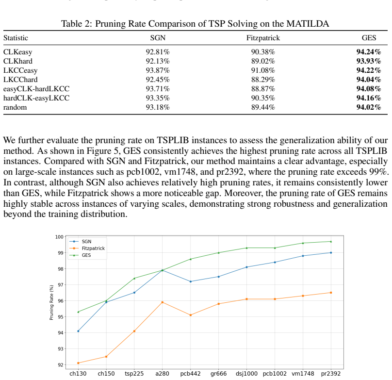
A GAT trained on Delaunay-prefiltered Euclidean TSP graphs, using four edge features (distance, KNN membership, iterative-MST weight, and local quality ratio) plus a Christofides safety net, produces sparse subgraphs that prune 95% of edges on 100-city MATILDA instances and over 99% on large TSPLIB instances while keeping the optimality gap of the subsequent exact solution under 1%.

What carries the argument

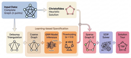
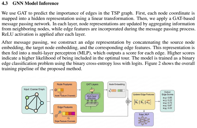
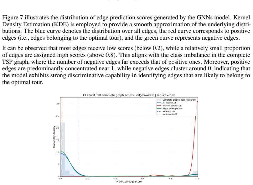
GES: Delaunay coarse graph → four-dimensional edge features → GATv2 edge scoring → threshold filter plus Christofides edges → exact solver on the residual sparse graph.

Load-bearing premise

That a model trained only on a fraction of 100-city MATILDA instances, with a fixed score threshold and Christofides augmentation, will keep a near-optimal tour’s edges on much larger and differently distributed TSPLIB cities.

What would settle it

Take any TSPLIB instance larger than pr2392 for which an optimal tour is known; run the published GES pipeline with the same threshold and check whether the sparse graph still contains a tour whose length is within 1% of that optimum.

Watch this falsifier — get emailed when new claim-graph text bears on it.

If this is right

Exact MIP solvers can be applied to TSP instances whose complete graphs were previously too large for memory.
The same learned candidate set can be handed to any heuristic (LKH, Christofides, etc.) to accelerate local search.
Because the model generalizes from 100-city training data to thousands of cities, a single trained sparsifier can serve as a reusable front-end for many Euclidean TSP solvers.
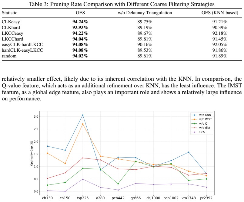
Ablation evidence shows that dropping the Delaunay pre-filter or any of the four edge features measurably worsens either pruning rate or optimality gap, so each component is necessary for the claimed performance.

Where Pith is reading between the lines

These are editorial extensions of the paper, not claims the author makes directly.

The same feature-plus-attention recipe may transfer to other geometric combinatorial problems (vehicle routing, Steiner trees) where short edges dominate high-quality solutions.
If the score threshold can be made adaptive to graph size or density, the method could avoid the residual infeasibility that currently forces Christofides edges on hard instances.
Because the model never sees the final tour during inference, it can be viewed as a learned, instance-specific replacement for classic candidate-set heuristics used inside LKH-style solvers.

Editorial analysis

A structured set of objections, weighed in public.

Desk editor's note, referee report, simulated authors' rebuttal, and a circularity audit.

Desk Editor's Note

Solid incremental sparsification pipeline with real empirical gains; threshold opacity and Christofides safety net are the main soft spots, not a collapse of the result.

read the letter

Punchline: this is a clean empirical systems paper that recombines known pieces—Delaunay coarse graph, engineered edge features, GATv2 scoring, Christofides feasibility edges—into a pipeline that beats Fitzpatrick and Xin on both pruning and optimality gap on MATILDA and TSPLIB. It is not a theory paper and not a conceptual leap; it is useful engineering for Euclidean TSP candidate sets.

What is actually new is the combined recipe and the measured outcomes, not any single ingredient. Delaunay as coarse filter, IMST-style and local quality features, and GNN edge scoring already exist. The paper’s contribution is showing that this particular stack, trained as supervised edge classification on ~100-node MATILDA splits, can prune ~94–95% on MATILDA with gaps often ~0.1–0.2% on hard sets, and on large TSPLIB instances push pruning past 99% while staying under 1% gap. Ablations on coarse filter (Table 3), features (Fig. 8 / Table 6), and Christofides feasibility (Table 7) are present and informative. The central empirical pattern is coherent: higher prune, lower gap, better speedup than the two baselines they chose.

Soft spots, in proportion. The score threshold is never stated numerically—that is a real reproducibility hole, not a nit. Training is on 100-node MATILDA subsets; the TSPLIB generalization claim is load-bearing and under-specified. Table 7 shows that without Christofides, hard MATILDA subsets already produce some infeasible graphs, so the safety net is doing real work for connectivity. The stress-test overreaches, though: Christofides alone is a 3/2 guarantee; gaps of ~0.1–0.3% on large instances cannot be explained by Christofides edges dominating the retained tour. The GAT is retaining useful structure; Christofides is mostly a feasibility patch. Free parameters (threshold, class weight 30, k, architecture) are many and not swept carefully. No code. Citation pattern is fine for the niche.

Who it is for: people who build or use candidate-edge sets for geometric TSP / exact or hybrid solvers. A learning-for-CO reading group gets a concrete pipeline and honest ablations; a theory group does not. Math is standard GAT + BCE; data story is external metrics against optima, not circular. I would send it to peer review—accept-shaped if they fix threshold reporting, release code/splits, and clarify how much of the tour is learned vs Christofides. Engage if you care about TSP sparsification baselines; skip if you need new theory.

Referee Report

4 major / 7 minor

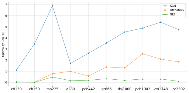
Summary. The paper proposes GES-TSP, a learning-based edge sparsification pipeline for Euclidean TSP. It first builds a Delaunay triangulation as a coarse candidate graph, constructs four edge features (Euclidean distance, binary KNN membership, a normalized iterative-MST score, and a local quality ratio Q_ij), scores edges with a GATv2 model trained as supervised binary classification against optimal tours, retains edges above a score threshold, and augments the sparse graph with Christofides edges to guarantee a feasible tour. The sparsified instance is then solved with SCIP. On MATILDA (100-node instances), the method reports pruning rates around 94% with optimality gaps typically well below 1%, outperforming SGN and Fitzpatrick baselines on both gap and pruning. On TSPLIB instances up to pr2392, it reports pruning rates above 99% on large instances with gaps remaining under 1%. Ablations address the coarse filter, individual features, and the Christofides augmentation.

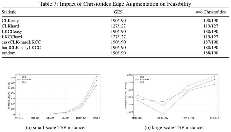
Significance. If the empirical claims hold under fully specified and fair evaluation, the work is a useful practical contribution to exact/high-quality TSP solving: it shows that a relatively light GAT, combined with classical geometric structure and a feasibility safety net, can discard the vast majority of edges while preserving near-optimal tours, with apparent transfer from 100-node training instances to larger TSPLIB graphs. Strengths include a clear modular pipeline, comparison against two relevant sparsification baselines, feature and coarse-filter ablations (Table 3, Fig. 8), a feasibility ablation for Christofides (Appendix Table 7), and consistent reporting of both pruning rate and optimality gap. The contribution is primarily empirical and engineering-oriented rather than theoretical; its value for the community depends on reproducibility of the sparsification rule and on clarifying how much of the reported quality comes from learned scores versus Delaunay structure and Christofides edges.

major comments (4)

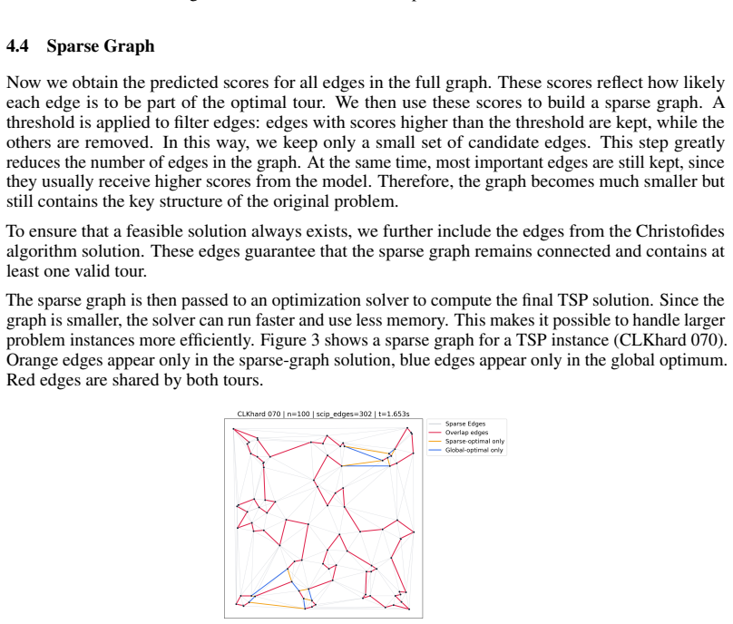
§4.4 (Sparse Graph) never states the numerical score threshold used to retain edges, nor whether it is fixed across instances, chosen by validation, or adjusted per graph size. This threshold is load-bearing for every pruning-rate and optimality-gap number in Tables 1–2, Figs. 4–5, and Appendix Tables 4–5. Without the value (or a selection procedure), the central results are not reproducible and the comparison of pruning rates against SGN (top-k) and Fitzpatrick is not fully interpretable.
§4.4 and Appendix Table 7: without Christofides augmentation, the pipeline already yields infeasible graphs on 8/127 CLKhard and 8/127 LKCChard instances—the hard distributions used in training. The TSPLIB “strong generalization” claim (pruning >99%, gap <1% after training only on ~100-node MATILDA subsets) therefore needs a quantitative breakdown of how many retained tour edges come from GAT scores versus forced Christofides edges, and of the gap when Christofides edges are excluded or replaced by a weaker connectivity fix. Otherwise it is unclear whether the headline generalization is driven by the learned sparsifier or by the 3/2-approximation safety net.
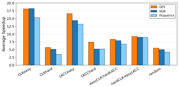
§5.1 comparative study: the paper does not fully specify how the SGN and Fitzpatrick baselines were configured for a fair head-to-head (e.g., k for SGN, decision threshold or feature set for Fitzpatrick, whether all three methods feed the same SCIP formulation and time limits, and whether GNN inference time is included in speedups in Fig. 6). Because pruning rate and gap trade off, unequal operating points could inflate GES’s advantage. Please report the exact baseline settings and, ideally, a gap-vs-pruning Pareto comparison.
§5 training setup and free parameters: the model is trained on one-third of CLKhard and LKCChard (100 nodes) with a fixed positive class weight of 30, GATv2 hyperparameters, and an unspecified KNN neighborhood size k in the edge features. The generalization premise to TSPLIB instances up to ~2400 nodes is central to the abstract and §6. A sensitivity analysis of threshold, k, and class weight—and at least one experiment training or validating on a different size/distribution—would substantially strengthen the claim that the GAT, not only Delaunay+Christofides, transfers.

minor comments (7)

Abstract and title block: missing space after period (“benchmark.In some”); affiliation typo “Lanzhou Universtiy” (twice).
§3.2 Eq. (1)–(2): notation mixes h_v and h^{(l)}_v; edge feature r_vu is introduced without defining how the four-dimensional e_ij of §4.2 is mapped into the attention input.
§4.2 Eq. (4): Q_ij uses min_k d_ik; clarify whether the min is over neighbors in the Delaunay graph or over all other nodes, and state the KNN parameter k used in Eq. (3).
§5: “we consider instances ranging from ch130 to pr2392, since optimal solution files are not available…” is a run-on sentence; also clarify that MATILDA categories each have 190 instances of size 100.
Figures 4–6 and 9: axis labels, units, and whether times include model inference vs. SCIP only should be stated in captions for readability.
Related work: end-to-end neural TSP methods are cited but the positioning relative to other learning-to-prune / candidate-set methods could briefly note differences in supervision and solver coupling.
Appendix Table 6 vs. main Fig. 8: feature-ablation gaps on TSPLIB are useful; ensure the main text points readers to the full table for exact numbers.

Circularity Check

0 steps flagged

No circularity: supervised edge classification trained on optimal tours and evaluated via independent external metrics (pruning rate, optimality gap) on held-out and out-of-distribution instances.

full rationale

The paper's pipeline is standard supervised learning for sparsification: Delaunay coarse graph + hand-crafted geometric features (distance, KNN, Q, normalized IMST) feed a GAT that is trained by binary cross-entropy against known optimal-tour edges on a MATILDA training split; a score threshold plus Christofides edges then produce a sparse graph that is solved by SCIP. All reported quantities (optimality gap to true optima, pruning rate relative to the complete graph, speed-up) are computed on held-out MATILDA categories and on external TSPLIB instances never seen during training. None of the six circularity patterns applies: there is no self-definitional equation, no fitted parameter re-labeled as a prediction of a dependent quantity, no load-bearing self-citation, no uniqueness theorem imported from the authors, no ansatz smuggled via self-citation, and no renaming of a known empirical pattern. Geometric facts (Delaunay, Christofides) are classical background, not circular inputs. The method is therefore self-contained against external benchmarks; any concerns about threshold choice or the Christofides safety net are generalization/correctness issues, not circularity.

Axiom & Free-Parameter Ledger

5 free parameters · 5 axioms · 2 invented entities

The central claims rest on empirical ML practice plus standard geometric/CO facts, not on new physical entities. Load-bearing free choices are the score threshold, class-weight, architecture, and training split; domain axioms are that Delaunay and local/global edge features carry near-optimal edges and that Christofides edges restore feasibility. No new particles or forces are postulated—only a named pipeline (GES) and a simplified Q feature.

free parameters (5)

edge score threshold for sparsification
§4.4 keeps edges above an unspecified threshold; pruning rate and feasibility depend on this choice, yet no value, selection rule, or sensitivity study is given.
BCE positive class weight
§5 sets positive weight 30 to handle class imbalance; this is a hand-chosen training hyperparameter that shapes predicted scores.
GAT architecture and training hyperparameters
3 GATv2 layers, hidden 64, 4 heads, lr 0.001, batch size 4, 50 epochs, dropout 0.1 are chosen by hand and determine the reported edge scores.
KNN neighborhood size k
KNN feature (§4.2) depends on k, which is not stated; feature ablation shows KNN is the most influential feature.
IMST iteration depth R=ceil(log2 n) and normalization
Global IMST feature construction and subsequent normalization are design choices that affect scale-invariance and edge ranking across sizes.

axioms (5)

domain assumption Delaunay triangulation retains many edges that appear in high-quality Euclidean TSP tours and is a sufficient O(n) coarse candidate set.
Invoked in §3.3 and §4.1 as the coarse graph; ablation Table 3 shows ~3–5% pruning drop without it.
standard math Christofides tour edges guarantee the sparsified graph contains at least one Hamiltonian cycle.
§3.4 and §4.4; Appendix Table 7 shows infeasible instances without this augmentation on hard sets.
domain assumption Optimal-tour edge labels on training instances are a valid supervision signal for predicting useful candidate edges on unseen instances.
Training as binary edge classification (§4.3, §5) assumes transfer of edge importance across instances and sizes.
domain assumption Euclidean distances and the four hand-crafted edge features (d, KNN, IMST, Q) are informative enough for GAT message passing to rank near-optimal edges.
Feature construction §4.2; ablations in Fig. 8 / Table 6 support contribution of each feature.
ad hoc to paper SCIP exact solutions on the sparsified graph are comparable across methods for reporting optimality gaps.
Experimental protocol §5 uses SCIP only; fairness depends on identical solver settings and baseline sparse graphs.

invented entities (2)

GES sparsification pipeline (Delaunay → GAT edge scores → threshold + Christofides) no independent evidence
purpose: Name and operationalize the end-to-end learned sparsifier claimed to beat prior learning-based sparsifiers.
Not a physical entity; a composite method. Independent evidence is only the paper’s own tables; no external replication yet.
Simplified local Q-value edge feature Q_ij = (1+d_ij)/(1+min_k d_ik) no independent evidence
purpose: Compress Fitzpatrick-style local features into one continuous local quality signal for the GNN.
Defined in §4.2; ablation shows small but positive effect. No external validation outside this paper.

pith-pipeline@v1.1.0-grok45 · 14055 in / 3676 out tokens · 46776 ms · 2026-07-14T17:24:46.052591+00:00 · methodology

0 comments

read the original abstract

Solving large-scale instances of the Traveling Salesman Problem (TSP) exactly is computationally expensive. Researchers often employ graph sparsification methods to improve computational efficiency. Traditional sparsification methods typically rely on fixed heuristics and fail to fully exploit instance-specific structural information. In this paper, we propose Graph Edge Sparsification (GES), a learning-based sparsification approach for Euclidean TSP. By incorporating geometric structural information and combinatorial optimization technology, our proposed method adaptively generates a sparsification graph for different instances, significantly reducing the graph size and accelerating the solving process. Experimental results demonstrate that our sparsification method can prune up to 95% of edges on the MATILDA dataset, while keeping the solution gap within 1% of the optimal value. Moreover, our approach exhibits strong generalization capability on the TSPLIB benchmark.In some large-scale instances, the pruning rate exceeds 99%, while the optimality gap remains below 1%.

Figures

Figures reproduced from arXiv: 2607.09708 by Tianfeng Chen, Xianyue Li.

**Figure 2.** Figure 2: Architecture of the Proposed GNNs Model 4.4 Sparse Graph Now we obtain the predicted scores for all edges in the full graph. These scores reflect how likely each edge is to be part of the optimal tour. We then use these scores to build a sparse graph. A threshold is applied to filter edges: edges with scores higher than the threshold are kept, while the others are removed. In this way, we keep only a small… view at source ↗

**Figure 3.** Figure 3: Sparse Graph for a TSP Instance 5 [PITH_FULL_IMAGE:figures/full_fig_p005_3.png] view at source ↗

**Figure 4.** Figure 4: Optimality Gap Comparison of TSP Solving on the TSPLIB [PITH_FULL_IMAGE:figures/full_fig_p007_4.png] view at source ↗

**Figure 5.** Figure 5: Pruning Rate Comparison of TSP Solving on the TSPLIB [PITH_FULL_IMAGE:figures/full_fig_p007_5.png] view at source ↗

**Figure 6.** Figure 6: Average speed-up on the MATILDA [PITH_FULL_IMAGE:figures/full_fig_p008_6.png] view at source ↗

**Figure 7.** Figure 7: illustrates the distribution of edge prediction scores generated by the GNNs model. Kernel Density Estimation (KDE) is employed to provide a smooth approximation of the underlying distributions. The blue curve denotes the distribution over all edges, the red curve corresponds to positive edges (i.e., edges belonging to the optimal tour), and the green curve represents negative edges. It can be observed th… view at source ↗

**Figure 8.** Figure 8: Ablation Results of Edge Features After selecting edges based on the threshold, we further incorporate the edges from the Christofides algorithm solution. As shown in [PITH_FULL_IMAGE:figures/full_fig_p009_8.png] view at source ↗

**Figure 9.** Figure 9: Comparison of running times on the TSPLIB [PITH_FULL_IMAGE:figures/full_fig_p013_9.png] view at source ↗

discussion (0)

Reference graph

Works this paper leans on

20 extracted references · 4 linked inside Pith

[1]

The traveling salesman problem

Michael Jünger, Gerhard Reinelt, and Giovanni Rinaldi. The traveling salesman problem. Handbooks in operations research and management science, 7:225–330, 1995

1995
[2]

Spectral sparsification of graphs.SIAM Journal on Computing, 40(4):981–1025, 2011

Daniel A Spielman and Shang-Hua Teng. Spectral sparsification of graphs.SIAM Journal on Computing, 40(4):981–1025, 2011

2011
[3]

Springer, 2008

Mark De Berg, Otfried Cheong, Marc Van Kreveld, and Mark Overmars.Computational geometry: algorithms and applications. Springer, 2008

2008
[4]

Xiangping Xu, Jun Li, and MengChu Zhou. Delaunay-triangulation-based variable neighbor- hood search to solve large-scale general colored traveling salesman problems.IEEE Transactions on Intelligent Transportation Systems, 22(3):1583–1593, 2020

2020
[5]

The transformer network for the traveling salesman problem.arXiv preprint arXiv:2103.03012, 2021

Xavier Bresson and Thomas Laurent. The transformer network for the traveling salesman problem.arXiv preprint arXiv:2103.03012, 2021

Pith/arXiv arXiv 2021
[6]

An efficient graph convolutional network technique for the travelling salesman problem.arXiv preprint arXiv:1906.01227, 2019

Chaitanya K Joshi, Thomas Laurent, and Xavier Bresson. An efficient graph convolutional network technique for the travelling salesman problem.arXiv preprint arXiv:1906.01227, 2019

Pith/arXiv arXiv 1906
[7]

Pointer networks.Advances in neural information processing systems, 28, 2015

Oriol Vinyals, Meire Fortunato, and Navdeep Jaitly. Pointer networks.Advances in neural information processing systems, 28, 2015

2015
[8]

Neural combina- torial optimization with reinforcement learning.arXiv preprint arXiv:1611.09940, 2016

Irwan Bello, Hieu Pham, Quoc V Le, Mohammad Norouzi, and Samy Bengio. Neural combina- torial optimization with reinforcement learning.arXiv preprint arXiv:1611.09940, 2016

Pith/arXiv arXiv 2016
[9]

Pomo: Policy optimization with multiple optima for reinforcement learning.Advances in neural information processing systems, 33:21188–21198, 2020

Yeong-Dae Kwon, Jinho Choo, Byoungjip Kim, Iljoo Yoon, Youngjune Gwon, and Seungjai Min. Pomo: Policy optimization with multiple optima for reinforcement learning.Advances in neural information processing systems, 33:21188–21198, 2020

2020
[10]

Learning to sparsify travelling salesman problem instances

James Fitzpatrick, Deepak Ajwani, and Paula Carroll. Learning to sparsify travelling salesman problem instances. InInternational Conference on Integration of Constraint Programming, Artificial Intelligence, and Operations Research, pages 410–426. Springer, 2021

2021
[11]

Liang Xin, Wen Song, Zhiguang Cao, and Jie Zhang. Neurolkh: Combining deep learning model with lin-kernighan-helsgaun heuristic for solving the traveling salesman problem.Advances in Neural Information Processing Systems, 34:7472–7483, 2021

2021
[12]

Combhelper: a neural approach to reduce search space for graph combinatorial problems

Hao Tian, Sourav Medya, and Wei Ye. Combhelper: a neural approach to reduce search space for graph combinatorial problems. InProceedings of the AAAI Conference on Artificial Intelligence, volume 38, pages 20812–20820, 2024

2024
[13]

A comprehensive survey on graph reduction: Sparsification, coarsening, and condensation

Mohammad Hashemi, Shengbo Gong, Juntong Ni, Wenqi Fan, B Aditya Prakash, and Wei Jin. A comprehensive survey on graph reduction: Sparsification, coarsening, and condensation. 2024

2024
[14]

The graph neural network model.IEEE transactions on neural networks, 20(1):61–80, 2008

Franco Scarselli, Marco Gori, Ah Chung Tsoi, Markus Hagenbuchner, and Gabriele Monfardini. The graph neural network model.IEEE transactions on neural networks, 20(1):61–80, 2008

2008
[15]

Open graph benchmark: Datasets for machine learning on graphs

Weihua Hu, Matthias Fey, Marinka Zitnik, Yuxiao Dong, Hongyu Ren, Bowen Liu, Michele Catasta, and Jure Leskovec. Open graph benchmark: Datasets for machine learning on graphs. Advances in neural information processing systems, 33:22118–22133, 2020

2020
[16]

Graph attention networks.stat, 1050:4, 2018

Petar Velickovic, Guillem Cucurull, Arantxa Casanova, Adriana Romero, Pietro Lio, and Yoshua Bengio. Graph attention networks.stat, 1050:4, 2018

2018
[17]

Worst-case analysis of a new heuristic for the travelling salesman problem

Nicos Christofides. Worst-case analysis of a new heuristic for the travelling salesman problem. InOperations Research Forum, volume 3, page 20. Springer, 2022

2022
[18]

Scip: solving constraint integer programs.Mathematical Programming Computation, 1(1):1–41, 2009

Tobias Achterberg. Scip: solving constraint integer programs.Mathematical Programming Computation, 1(1):1–41, 2009

2009
[19]

Solving the equality generalized traveling salesman problem using the lin– kernighan–helsgaun algorithm.Mathematical Programming Computation, 7(3):269–287, 2015

Keld Helsgaun. Solving the equality generalized traveling salesman problem using the lin– kernighan–helsgaun algorithm.Mathematical Programming Computation, 7(3):269–287, 2015. 10

2015
[20]

Generalization of machine learn- ing for problem reduction: a case study on travelling salesman problems.arXiv preprint arXiv:2005.05847, 2020

Yuan Sun, Andreas Ernst, Xiaodong Li, and Jake Weiner. Generalization of machine learn- ing for problem reduction: a case study on travelling salesman problems.arXiv preprint arXiv:2005.05847, 2020. 11 A Technical Appendices and Supplementary Material This appendix supplements the line charts in the main text by reporting the corresponding detailed numeri...

Pith/arXiv arXiv 2005

[1] [1]

The traveling salesman problem

Michael Jünger, Gerhard Reinelt, and Giovanni Rinaldi. The traveling salesman problem. Handbooks in operations research and management science, 7:225–330, 1995

1995

[2] [2]

Spectral sparsification of graphs.SIAM Journal on Computing, 40(4):981–1025, 2011

Daniel A Spielman and Shang-Hua Teng. Spectral sparsification of graphs.SIAM Journal on Computing, 40(4):981–1025, 2011

2011

[3] [3]

Springer, 2008

Mark De Berg, Otfried Cheong, Marc Van Kreveld, and Mark Overmars.Computational geometry: algorithms and applications. Springer, 2008

2008

[4] [4]

Xiangping Xu, Jun Li, and MengChu Zhou. Delaunay-triangulation-based variable neighbor- hood search to solve large-scale general colored traveling salesman problems.IEEE Transactions on Intelligent Transportation Systems, 22(3):1583–1593, 2020

2020

[5] [5]

The transformer network for the traveling salesman problem.arXiv preprint arXiv:2103.03012, 2021

Xavier Bresson and Thomas Laurent. The transformer network for the traveling salesman problem.arXiv preprint arXiv:2103.03012, 2021

Pith/arXiv arXiv 2021

[6] [6]

An efficient graph convolutional network technique for the travelling salesman problem.arXiv preprint arXiv:1906.01227, 2019

Chaitanya K Joshi, Thomas Laurent, and Xavier Bresson. An efficient graph convolutional network technique for the travelling salesman problem.arXiv preprint arXiv:1906.01227, 2019

Pith/arXiv arXiv 1906

[7] [7]

Pointer networks.Advances in neural information processing systems, 28, 2015

Oriol Vinyals, Meire Fortunato, and Navdeep Jaitly. Pointer networks.Advances in neural information processing systems, 28, 2015

2015

[8] [8]

Neural combina- torial optimization with reinforcement learning.arXiv preprint arXiv:1611.09940, 2016

Irwan Bello, Hieu Pham, Quoc V Le, Mohammad Norouzi, and Samy Bengio. Neural combina- torial optimization with reinforcement learning.arXiv preprint arXiv:1611.09940, 2016

Pith/arXiv arXiv 2016

[9] [9]

Pomo: Policy optimization with multiple optima for reinforcement learning.Advances in neural information processing systems, 33:21188–21198, 2020

Yeong-Dae Kwon, Jinho Choo, Byoungjip Kim, Iljoo Yoon, Youngjune Gwon, and Seungjai Min. Pomo: Policy optimization with multiple optima for reinforcement learning.Advances in neural information processing systems, 33:21188–21198, 2020

2020

[10] [10]

Learning to sparsify travelling salesman problem instances

James Fitzpatrick, Deepak Ajwani, and Paula Carroll. Learning to sparsify travelling salesman problem instances. InInternational Conference on Integration of Constraint Programming, Artificial Intelligence, and Operations Research, pages 410–426. Springer, 2021

2021

[11] [11]

Liang Xin, Wen Song, Zhiguang Cao, and Jie Zhang. Neurolkh: Combining deep learning model with lin-kernighan-helsgaun heuristic for solving the traveling salesman problem.Advances in Neural Information Processing Systems, 34:7472–7483, 2021

2021

[12] [12]

Combhelper: a neural approach to reduce search space for graph combinatorial problems

Hao Tian, Sourav Medya, and Wei Ye. Combhelper: a neural approach to reduce search space for graph combinatorial problems. InProceedings of the AAAI Conference on Artificial Intelligence, volume 38, pages 20812–20820, 2024

2024

[13] [13]

A comprehensive survey on graph reduction: Sparsification, coarsening, and condensation

Mohammad Hashemi, Shengbo Gong, Juntong Ni, Wenqi Fan, B Aditya Prakash, and Wei Jin. A comprehensive survey on graph reduction: Sparsification, coarsening, and condensation. 2024

2024

[14] [14]

The graph neural network model.IEEE transactions on neural networks, 20(1):61–80, 2008

Franco Scarselli, Marco Gori, Ah Chung Tsoi, Markus Hagenbuchner, and Gabriele Monfardini. The graph neural network model.IEEE transactions on neural networks, 20(1):61–80, 2008

2008

[15] [15]

Open graph benchmark: Datasets for machine learning on graphs

Weihua Hu, Matthias Fey, Marinka Zitnik, Yuxiao Dong, Hongyu Ren, Bowen Liu, Michele Catasta, and Jure Leskovec. Open graph benchmark: Datasets for machine learning on graphs. Advances in neural information processing systems, 33:22118–22133, 2020

2020

[16] [16]

Graph attention networks.stat, 1050:4, 2018

Petar Velickovic, Guillem Cucurull, Arantxa Casanova, Adriana Romero, Pietro Lio, and Yoshua Bengio. Graph attention networks.stat, 1050:4, 2018

2018

[17] [17]

Worst-case analysis of a new heuristic for the travelling salesman problem

Nicos Christofides. Worst-case analysis of a new heuristic for the travelling salesman problem. InOperations Research Forum, volume 3, page 20. Springer, 2022

2022

[18] [18]

Scip: solving constraint integer programs.Mathematical Programming Computation, 1(1):1–41, 2009

Tobias Achterberg. Scip: solving constraint integer programs.Mathematical Programming Computation, 1(1):1–41, 2009

2009

[19] [19]

Solving the equality generalized traveling salesman problem using the lin– kernighan–helsgaun algorithm.Mathematical Programming Computation, 7(3):269–287, 2015

Keld Helsgaun. Solving the equality generalized traveling salesman problem using the lin– kernighan–helsgaun algorithm.Mathematical Programming Computation, 7(3):269–287, 2015. 10

2015

[20] [20]

Generalization of machine learn- ing for problem reduction: a case study on travelling salesman problems.arXiv preprint arXiv:2005.05847, 2020

Yuan Sun, Andreas Ernst, Xiaodong Li, and Jake Weiner. Generalization of machine learn- ing for problem reduction: a case study on travelling salesman problems.arXiv preprint arXiv:2005.05847, 2020. 11 A Technical Appendices and Supplementary Material This appendix supplements the line charts in the main text by reporting the corresponding detailed numeri...

Pith/arXiv arXiv 2005