REVIEW 4 major objections 4 minor 67 references
The paper proposes encoding a dataset's higher-order topology into a quantum state by evolving a uniform simplex state under the combinatorial Laplacian, and reports that this representation separates random-graph clique complexes more accu
Reviewed by Pith at T0; open to challenge. T0 means a machine referee read the full paper against a public rubric. the ladder, T0–T4 →
T0 review · deepseek-v4-flash
2026-08-02 03:31 UTC pith:3PVUYFV6
load-bearing objection A coherent but modest extension of quantum evolution kernels to higher-order Laplacians; the empirical advantage is underdetermined because the evolution time t is never reported and the QSVT gains are admitted to be selection-biased. the 4 major comments →
Quantum Topological Data Encoding
The pith
A machine-rendered reading of the paper's core claim, the machinery that carries it, and where it could break.
Core claim
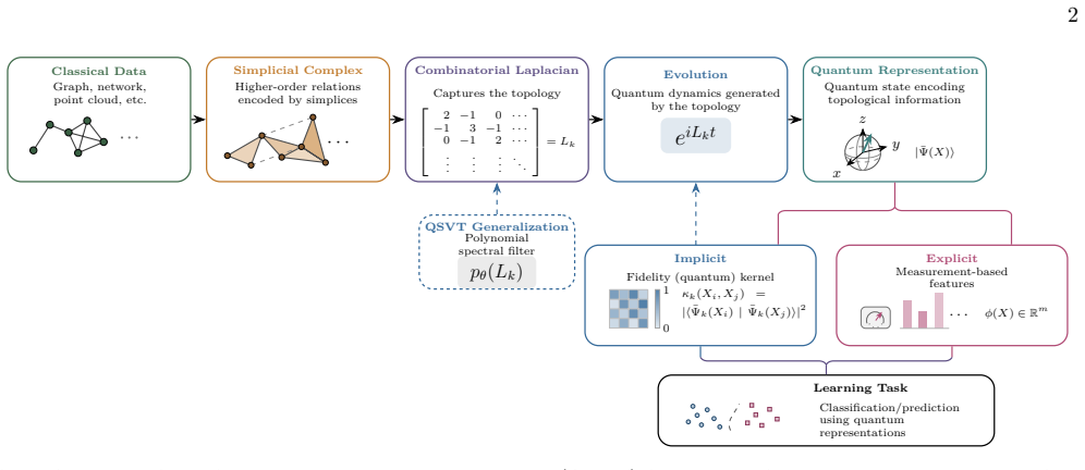
On its own terms, the paper claims that a data structure's k-th order topology can be encoded as |Ψ_k(X)⟩ = e^{-i L_k t}|s⟩, where L_k is the combinatorial Laplacian on k-simplices and |s⟩ is the uniform state over simplices. It defines an implicit quantum kernel from state fidelity and an explicit feature vector from survival amplitudes a(t) = ⟨s|e^{-iL_k t}|s⟩ sampled over time. On clique complexes of random graphs with different edge densities, the authors report that these quantum representations separate classes more accurately than a Gaussian kernel on the Euclidean distance between Laplacian matrices, with the largest advantage appearing at higher simplicial dimensions, and that the e
What carries the argument
The key object is the k-th combinatorial Laplacian L_k = B_k^T B_k + B_{k+1}B_{k+1}^T on a simplicial complex: the down term couples k-simplices through shared (k−1)-faces and the up term through shared (k+1)-cofaces. Because L_k is Hermitian and sparse, the exponential e^{-iL_k t} is a unitary driven by the topology, and the uniform state |s⟩ evolved under it carries the Laplacian's spectrum. The fidelity kernel |⟨Ψ(X_1)|Ψ(X_2)⟩|^2 and the survival features ⟨s|e^{-iL_k t_j}|s⟩ turn that spectrum into similarity scores; quantum singular value transformation lets the exponential be replaced by a trainable polynomial p(L_k) to emphasize selected spectral regions.
Load-bearing premise
The encoding's usefulness rests on the choice of evolution time t, which the paper refers to as 'some sufficiently large choice' and never fixes; if t is tuned per dataset to maximize accuracy, the claimed advantage is a fitting artifact rather than a property of the representation.
What would settle it
Re-run the benchmark with a fixed, disclosed evolution-time schedule (same t and time grid for every graph in both classes) and with the classical Laplacian baseline given the same hyperparameter tuning; if the quantum representations no longer lead, the central comparison is not robust.
If this is right
- Higher-order topological structure can be injected into quantum kernels and feature vectors without first computing Betti numbers or persistence diagrams.
- The explicit survival features give a low-dimensional, measurement-based readout that may be implementable with fewer resources than full state tomography.
- The discriminative topology of a dataset lives at a task-dependent simplicial dimension; QTDE motivates evaluating multiple k rather than a single fixed scale.
- Trainable polynomial spectral filters through quantum singular value transformation provide a mechanism to amplify or suppress spectral regions of the Laplacian to improve classification.
- Because the quantum representations are built from the Laplacian spectrum, they inherit invariance to vertex relabeling once the simplicial complex is fixed.
Where Pith is reading between the lines
- Not claimed by the paper: because the fidelity kernel and survival features depend on the Laplacian spectrum, two complexes with identical spectra but different homology would look identical to QTDE; a spectral-invariant test would clarify how much topology beyond the spectrum is actually being captured.
- Not claimed by the paper: the reported advantage may be sensitive to how the evolution time and time grid are set; if those are optimized per dataset, the comparison is fitted, and a fixed, disclosed schedule is needed to confirm the qualitative ranking.
- Not claimed by the paper: the zero-padding used to align complexes of different sizes introduces a dependence on the particular sample fleet; a normalization independent of the dataset's composition would make the kernel more portable.
- Not claimed by the paper: the framework suggests a natural extension to persistent Laplacians—evolving over a filtration and reading survival amplitudes at multiple scales could give a quantum persistence fingerprint.
Editorial analysis
A structured set of objections, weighed in public.
Referee Report
Summary. The paper introduces Quantum Topological Data Encoding (QTDE), a framework that maps a simplicial complex to a quantum state by evolving a uniform superposition over k-simplices under the unitary generated by the combinatorial Laplacian L_k. Two readouts are proposed: an implicit fidelity kernel between evolved states and an explicit feature vector formed from survival amplitudes sampled at multiple times. A generalization based on QSVT replaces the exponential by polynomial spectral filters. The method is evaluated on binary classification of clique complexes of Erdős–Rényi graphs, against a Gaussian kernel on Frobenius distances between Laplacians. The paper claims that the quantum representations 'consistently outperform' this classical baseline and that higher-dimensional Laplacians provide discriminative information not available from direct matrix comparisons.
Significance. If the empirical claims were fully supported, QTDE would be a useful proof-of-concept for topology-driven quantum encodings: the fidelity kernel is valid (PSD by the Schur product theorem), the survival features are a compact spectral fingerprint, and the extension to QSVT is technically natural. The manuscript also includes a welcome degree of self-criticism, especially in Sec. V.D and Sec. VII, and promises a public code repository, which would aid reproducibility. However, the central advantage claim currently rests on unreported evolution times and on per-dimension best-filter selection, both of which can turn a fitted curve into an apparent prediction. The paper's own admission that the QSVT advantages fall within the cross-validation spread further weakens the 'consistently outperform' statement. The contribution is therefore a promising framework whose empirical validation is not yet complete.
major comments (4)
- [Sec. III.B, Eq. (7) and Eq. (14); Sec. IV.C, Eq. (16)] The evolution time t and the time grid {t_j} are never reported. The text only states that t is 'some sufficiently large choice' (Sec. III.B). Both the fidelity kernel (Eq. 9) and the survival features (Eq. 14) depend on t and on the sampled times. Since quantities like |<s|e^{-iL_1 t}e^{iL_2 t}|s>|^2 are quasiperiodic in t, different t values can change which classes appear similar. If t was chosen per dataset or per dimension to maximize cross-validated accuracy, the reported advantage is fitted rather than predicted. Please report the exact t and grid used for every experiment, and provide either a sensitivity analysis over t or a nested cross-validation procedure that selects t on the training folds only. Without this, the central empirical claim is underdetermined.
- [Sec. V.A and Abstract] The abstract and Sec. VII state that QTDE 'consistently outperform[s]' the Laplacian-comparison baseline, but Sec. V.A reports that on the two hard ensembles, G(30,0.78 vs 0.80) and G(50,0.69 vs 0.70), the fidelity kernel, survival features, and matrix-difference baseline interleave within the 0.5–0.7 band and the separations are comparable to the cross-validation spread. The visible advantage occurs mainly on the easily separable G(50,0.60 vs 0.70) panel at higher k. The claim should be qualified to match the evidence, e.g., 'in some regimes', and supported by a statistical comparison across folds or a paired significance test rather than by inspection of overlapping error bars.
- [Sec. V.C and Sec. V.D] The QSVT 'best poly' curves in Fig. 4(a) are obtained by selecting, at each dimension k, the best-performing polynomial from a fixed library. Sec. V.D explicitly acknowledges that taking the maximum over the family 'inflates the reported values' and that the residual advantages 'fall within the cross-validation spread'. This is a selection-bias problem of exactly the kind that affects the choice of t. To substantiate the Sec. V.C claim that polynomial filters 'sit consistently above' the exponential evolution and the baseline, the evaluation must select the polynomial within the training folds (nested CV) or pre-register the polynomial family, and report the resulting distribution rather than the per-dimension maximum.
- [Sec. III.B1] The zero-padding procedure for complexes with different numbers of k-simplices makes the representation dataset-dependent. The states are embedded in a common Hilbert space whose dimension is determined by the union of simplices across the whole dataset, so the kernel value K_k(X1,X2) in Eq. (9) is not a function of the two data points alone but depends on which other graphs happen to be in the sample. The Frobenius baseline (Eq. 17) shares the same dataset-dependent common basis, so the comparison is fair, but the manuscript should acknowledge this dependence and test its stability, for example by subsampling the dataset and checking whether the kernel geometry and classification results change.
minor comments (4)
- [Abstract / Sec. VII] The phrase 'consistently outperform' is stronger than the evidence in Sec. V.A and should be softened to reflect the regimes in which the advantage actually appears.
- [Sec. II.C and Sec. III.B] The sign convention for the evolution operator is inconsistent: Eq. (5) defines U_k(t)=e^{iL_k t} and Eq. (7) uses e^{iL_k t}|s>, while the introductory Eq. (1) and the kernel Eq. (9) write e^{-iL_k t}. The states are related by time reversal, but the inconsistency should be fixed for clarity.
- [Fig. 3 caption] The caption says 'cyan lines indicate the class boundary' while the Appendix captions for Figs. 6–7 refer to a 'cyan cross'. Please make the marker description consistent.
- [Sec. IV.C] The normalization constant c_k = max_G(max diag(L_k(G))) is described verbally but the actual values are not reported. Since all Laplacians are scaled by this dataset-wide constant, reporting c_k for each benchmark would aid reproducibility.
Circularity Check
A non-central QSVT best-polynomial curve is a fitted maximum (explicitly conceded), while the main exponential-QTDE vs Laplacian comparison is self-contained.
specific steps
-
fitted input called prediction
[Sec. V.C (Fig. 4a) and Sec. V.D; see also Sec. V.E]
"Selecting, at each k, the best-performing polynomial from the library (QSVT-fidelity, best poly and QSVT-survival, best poly) produces a curve that sits consistently above both the original exponential fidelity/survival kernels and the matrix-difference baseline ... These QSVT scores are, moreover, the maximum accuracy over a family of polynomials at each k. This selection bias inflates the reported values, so the residual advantages fall within the cross-validation spread."
The 'QSVT outperforms exponential' curve is not the accuracy of a fixed representation: at every k it is the maximum over ten polynomial filters evaluated on the same cross-validation folds. A per-fold maximum is upward-biased relative to any single fixed filter, so the reported separation from the exponential and matrix-difference baselines is partly an artifact of selecting the best filter after seeing validation labels. This is equivalent to fitting the filter choice to the test folds and then presenting the selected maximum as a predictive advantage. The paper concedes the inflation in Sec. V.D, yet Sec. V.C and Sec. V.E still read the selected-max curve as evidence that polynomial filters 'consistently outperform' the exponential evolution.
full rationale
The main exponential-QTDE vs Laplacian-baseline comparison is not circular by construction: both methods consume the same combinatorial Laplacian L_k (Eqs. 9 and 17), and no equation identifies the fidelity kernel or survival features with the Frobenius baseline. The generalization from QEK [52] is an external, acknowledged starting point; there is no load-bearing self-citation (the only coauthor self-citation, Ref. [31], is background) and no uniqueness theorem imported. The QSVT section contains the one reduction-by-construction step scored above: the best-polynomial curve is a fitted maximum, and the authors explicitly admit the selection bias. This is partial circularity of a secondary claim, not of the main representation. Separately, the evolution time t is left as 'some sufficiently large choice' (Sec. III.B) and the grid {t_j} is not reported (Sec. IV.C); this is an unresolved reproducibility/selection risk that could hide fitting of the central QTDE-vs-baseline result, but the paper's text supplies no explicit reduction showing t is fitted, so I do not score it as a demonstrated circular step. The paper's own limitations ('we do not provide formal guarantees', 'precise origin of this advantage is not yet fully understood') further weigh against a charge of hidden circularity in the core derivation.
Axiom & Free-Parameter Ledger
free parameters (3)
- evolution time t (or time grid {t_j}) =
not reported
- per-dimension best QSVT polynomial filter =
library of ten polys; best per k (e.g., x^2, 2x+x^2)
- survival feature sampling times {t_j} and count T =
not reported
axioms (5)
- ad hoc to paper Suitable evolution time t exists making the topology-driven states class-discriminative
- domain assumption Uniform superposition |s⟩ probes the Laplacian spectrum sufficiently
- domain assumption Zero-padding is a valid common embedding across complexes of different sizes
- domain assumption Combinatorial Laplacian spectral information is discriminative for the benchmark at all k
- standard math QSVT block-encoding and polynomial filtering can be implemented at the stated cost
read the original abstract
Many datasets encountered across a wide range of domains possess rich geometric and topological structure that is difficult to capture using conventional vector-based representations. Quantum machine learning offers the possibility of processing high-dimensional data in Hilbert spaces, but its practical success depends critically on how classical data is encoded into quantum states. We introduce \emph{quantum topological data encoding} (QTDE), a general framework for encoding topological information into quantum states via topology-driven quantum evolution. Our method generalises an existing topology-driven quantum encoding framework to higher-dimensional data. We test the proposed method on clique-complexes classification tasks, and provide preliminary evidence that topology-driven quantum representations can capture discriminative information beyond that available through direct comparisons of classical topological descriptors. The proposed quantum representations consistently outperform a baseline based on direct comparisons of the combinatorial Laplacians describing the underlying topological structure. We indicate several areas of application where the framework can be used to provide a more efficient and reliable data representation.
Figures


Reference graph
Works this paper leans on
-
[1]
Clique Complexes For each graphG we take itsclique(or flag) complex K(G): the simplicial complex whosek-simplices are the (k+1)-cliques of G, so that an edge is a1-simplex, a triangle a2-simplex, a tetrahedron a3-simplex, and so on. The clique complex is determined entirely by the graph’s edge set, namely a set of vertices spans a simplex whenever they ar...
-
[2]
The map is a genuine feature map: the (in general high-dimensional) vector|Ψk(X)⟩ is never materialised explicitly and is accessed only through inner products
Implicit Representation: Topological Quantum Kernel We define the feature mapK(X)↦→Hthat sends the complex to the quantum state obtained by evolving a fixed reference state|s⟩ under the topology-driven unitary (5), |Ψk(X)⟩=U k(t)|s⟩=e iLkt|s⟩,|s⟩∈C nk,(7) where|s⟩ is the uniform superposition state over the simplices in the complex; |s⟩= 1√nk nk∑ i=1 |i⟩....
-
[3]
The second representation instead summarises the same evolution by a small number of measurement outcomes, yielding an explicit feature vector amenable to a linear model
Explicit Representation: Measurement Features The implicit representation requires the full state and a pairwise kernel. The second representation instead summarises the same evolution by a small number of measurement outcomes, yielding an explicit feature vector amenable to a linear model. Starting from a fixed initial state|s⟩(Equation (8)) on thek-simp...
2026
-
[4]
C. M. Bishop,Pattern Recognition and Machine Learning (Springer, New York, NY, 2006)
2006
-
[5]
K. P. Murphy,Machine learning: a probabilistic perspec- tive(MIT press, 2012)
2012
-
[6]
Goodfellow, Y
I. Goodfellow, Y. Bengio, and A. Courville,Deep Learning (MIT Press, 2016)http://www.deeplearningbook.org
2016
-
[7]
Manin,Mathematics as Metaphor: Selected Essays of Yuri I
I. Manin,Mathematics as Metaphor: Selected Essays of Yuri I. Manin, [Collected works (American Mathematical Society) (American Mathematical Society, 2007)
2007
-
[8]
P. Benioff, The computer as a physical system: A micro- scopic quantum mechanical hamiltonian model of com- puters as represented by turing machines, Journal of Sta- tistical Physics22, 563 (1980)
1980
-
[9]
R. P. Feynman, Simulating physics with computers, Inter- national Journal of Theoretical Physics21, 467 (1982)
1982
-
[10]
Aïmeur, G
E. Aïmeur, G. Brassard, and S. Gambs, Machine learning in a quantum world, inAdvances in Artificial Intelligence, edited by L. Lamontagne and M. Marchand (Springer Berlin Heidelberg, Berlin, Heidelberg, 2006) pp. 431–442
2006
-
[11]
Dunjko, J
V. Dunjko, J. M. Taylor, and H. J. Briegel, Quantum- enhanced machine learning, Phys. Rev. Lett.117, 130501 (2016)
2016
-
[12]
Dunjko and H
V. Dunjko and H. J. Briegel, Machine learning & ar- tificial intelligence in the quantum domain: a review of recent progress, Reports on Progress in Physics81, 074001 (2018)
2018
-
[13]
K. Beer, D. Bondarenko, T. Farrelly, T. J. Osborne, R. Salzmann, D. Scheiermann, and R. Wolf, Training deep quantum neural networks, Nature Communications 11, 10.1038/s41467-020-14454-2 (2020)
-
[14]
S. Y. Chang and M. Cerezo, A primer on quantum ma- chine learning (2025), arXiv:2511.15969 [quant-ph]
arXiv 2025
-
[15]
Schuld and F
M. Schuld and F. Petruccione,Machine Learning with Quantum Computers, Quantum Science and Technology (Springer International Publishing, 2021)
2021
-
[16]
LaRose and B
R. LaRose and B. Coyle, Robust data encodings for quan- tum classifiers, Physical Review A102(2020)
2020
-
[17]
S. Lloyd, M. Schuld, A. Ijaz, J. Izaac, and N. Killo- ran, Quantum embeddings for machine learning (2020), arXiv:2001.03622 [quant-ph]
Pith/arXiv arXiv 2020
-
[18]
Pérez-Salinas, A
A. Pérez-Salinas, A. Cervera-Lierta, E. Gil-Fuster, and J. I. Latorre, Data re-uploading for a universal quantum classifier, Quantum4, 226 (2020)
2020
-
[19]
T. Hur, I. F. Araujo, and D. K. Park, Neural quantum embedding: Pushing the limits of quantum supervised learning, Phys. Rev. A110, 022411 (2024)
2024
-
[20]
S. Shin, Y. S. Teo, and H. Jeong, Exponential data encod- ing for quantum supervised learning, Phys. Rev. A107, 012422 (2023)
2023
-
[21]
M. C. Caro, E. Gil-Fuster, J. J. Meyer, J. Eisert, and R. Sweke, Encoding-dependent generalization bounds for parametrized quantum circuits, Quantum5, 582 (2021)
2021
-
[22]
C. Lee, I. F. Araujo, D. Kim, J. Lee, S. Park, J.-Y. Ryu, and D. K. Park, Optimizing quantum convolutional neural network architectures for arbitrary data dimension, Fron- tiers in Physics13, 10.3389/fphy.2025.1529188 (2025)
arXiv 2025
-
[23]
O. Zang, G. Barrué, and T. Quertier, Benchmarking data encoding methods in quantum machine learning (2025), arXiv:2505.14295 [quant-ph]
arXiv 2025
-
[24]
Havlíček, A
V. Havlíček, A. D. Córcoles, K. Temme, A. W. Harrow, A. Kandala, J. M. Chow, and J. M. Gambetta, Supervised learning with quantum-enhanced feature spaces, Nature 567, 209 (2019)
2019
-
[25]
Schuld and N
M. Schuld and N. Killoran, Quantum machine learning in feature Hilbert spaces, Physical Review Letters122 (2019)
2019
-
[26]
Jäger, P
J. Jäger, P. Elsässer, and E. Torabian, Quantum feature- map learning with reduced resource overhead, Phys. Rev. Res.8, 023247 (2026)
2026
-
[27]
S. C. Marshall, C. Gyurik, and V. Dunjko, High Dimen- sional Quantum Machine Learning With Small Quantum Computers, Quantum7, 1078 (2023)
2023
-
[28]
M. Schuld, Supervised quantum machine learning models are kernel methods (2021), arXiv:2101.11020 [quant-ph]
Pith/arXiv arXiv 2021
-
[29]
J. Tanner, C.-F. Kam, and J. Wang, Non-variational supervised quantum kernel methods: a review (2026), arXiv:2604.07896 [quant-ph]
Pith/arXiv arXiv 2026
-
[30]
Carlsson, Topology and data, Bulletin of the American Mathematical Society46, 255 (2009)
G. Carlsson, Topology and data, Bulletin of the American Mathematical Society46, 255 (2009)
2009
-
[31]
Edelsbrunner and J
H. Edelsbrunner and J. Harer,Computational Topology: An Introduction, Applied Mathematics (American Mathe- matical Society, 2010)
2010
-
[32]
Carlsson, Topological methods for data modelling, Nature Reviews Physics2, 697 (2020)
G. Carlsson, Topological methods for data modelling, Nature Reviews Physics2, 697 (2020)
2020
-
[33]
Chazal and B
F. Chazal and B. Michel, An introduction to topological data analysis: fundamental and practical aspects for data scientists, Frontiers in artificial intelligence4, 667963 (2021)
2021
-
[34]
Leykam and D
D. Leykam and D. G. Angelakis, Topological data analysis and machine learning, Advances in Physics: X8, 2202331 (2023). 14
2023
-
[35]
Scali, C
S. Scali, C. Umeano, and O. Kyriienko, Quantum topo- logical data analysis via the estimation of the density of states, Physical Review A110(2024)
2024
-
[36]
Carlsson and M
G. Carlsson and M. Vejdemo-Johansson,Topological data analysis with applications(Cambridge University Press, 2021)
2021
-
[37]
A. Ta-Shma, Inverting well conditioned matrices in quan- tum logspace, inProceedings of the Forty-Fifth Annual ACM Symposium on Theory of Computing, STOC ’13 (Association for Computing Machinery, New York, NY, USA, 2013) p. 881–890
2013
-
[38]
C. M. Topaz, L. Ziegelmeier, and T. Halverson, Topologi- cal data analysis of biological aggregation models, PloS one10, e0126383 (2015)
2015
-
[39]
Wu and X
I. Wu and X. Wang, A novel approach to topological network analysis for the identification of metrics and signatures in non-small cell lung cancer, Scientific Reports 13, 8223 (2023)
2023
-
[40]
P. Y. Lum, G. Singh, A. Lehman, T. Ishkanov, M. Vejdemo-Johansson, M. Alagappan, J. Carlsson, and G. Carlsson, Extracting insights from the shape of com- plex data using topology, Scientific Reports3, 1236 (2013)
2013
-
[41]
Rabadán, Y
R. Rabadán, Y. Mohamedi, U. Rubin, T. Chu, A. N. Alghalith, O. Elliott, L. Arnés, S. Cal, Á. J. Obaya, A. J. Levine,et al., Identification of relevant genetic alterations in cancer using topological data analysis, Nature Commu- nications11, 3808 (2020)
2020
-
[42]
Nicolau, A
M. Nicolau, A. J. Levine, and G. Carlsson, Topology based data analysis identifies a subgroup of breast cancers with a unique mutational profile and excellent survival, Proceedings of the National Academy of Sciences108, 7265 (2011)
2011
-
[43]
Singh, C
Y. Singh, C. M. Farrelly, Q. A. Hathaway, T. Leiner, J. Jagtap, G. E. Carlsson, and B. J. Erickson, Topological data analysis in medical imaging: current state of the art, Insights into Imaging14, 58 (2023)
2023
-
[44]
Lloyd, S
S. Lloyd, S. Garnerone, and P. Zanardi, Quantum al- gorithms for topological and geometric analysis of data, Nature Communications7, 10138 (2016)
2016
-
[45]
Hayakawa, Quantum algorithm for persistent Betti numbers and topological data analysis, Quantum6, 873 (2022)
R. Hayakawa, Quantum algorithm for persistent Betti numbers and topological data analysis, Quantum6, 873 (2022)
2022
-
[46]
D. W. Berry, Y. Su, C. Gyurik, R. King, J. Basso, A. D. T. Barba, A. Rajput, N. Wiebe, V. Dunjko, and R. Babbush, Analyzing prospects for quantum advantage in topological data analysis, PRX Quantum5, 010319 (2024)
2024
-
[47]
Incudini, F
M. Incudini, F. Martini, and A. Di Pierro, Higher-order topological kernels via quantum computation, in2023 IEEE International Conference on Quantum Computing and Engineering (QCE), Vol. 01 (2023) pp. 621–629
2023
-
[48]
Gyurik, C
C. Gyurik, C. Cade, and V. Dunjko, Towards quantum advantage via topological data analysis, Quantum6, 855 (2022)
2022
-
[49]
S. Ubaru, I. Y. Akhalwaya, M. S. Squillante, K. L. Clark- son, and L. Horesh, Quantum topological data analy- sis with linear depth and exponential speedup (2021), arXiv:2108.02811 [quant-ph]
Pith/arXiv arXiv 2021
-
[50]
C. Gyurik, A. Schmidhuber, R. King, V. Dunjko, and R. Hayakawa, Provable quantum speedups for computing persistence in topological data analysis, PRX Quantum 7, 10.1103/gvys-hl8h (2026)
-
[51]
McArdle, A
S. McArdle, A. Gilyén, and M. Berta, A streamlined quantum algorithm for topological data analysis with exponentially fewer qubits, Quantum10, 2058 (2026)
2058
-
[52]
N.A.Nghiem,Towardsquantumtopologicaldataanalysis: torsion detection (2025), arXiv:2508.19943 [quant-ph]
arXiv 2025
-
[53]
Comput.20, 375 (2019)
R.Mengoni, A.D.Pierro, L.Memarzadeh,andS.Mancini, Persistent homology analysis of multiqubit entanglement, Quantum Inf. Comput.20, 375 (2019)
2019
-
[54]
M. Schuld, R. Sweke, and J. J. Meyer, The effect of data encoding on the expressive power of variational quantum- machine-learning models, Physical Review A103, 032430 (2021), arXiv:2008.08605 [quant-ph]
Pith/arXiv arXiv 2021
-
[55]
Henry, S
L.-P. Henry, S. Thabet, C. Dalyac, and L. Henriet, Quan- tum evolution kernel: Machine learning on graphs with programmable arrays of qubits, Phys. Rev. A104, 032416 (2021)
2021
-
[56]
Gilyén, Y
A. Gilyén, Y. Su, G. H. Low, and N. Wiebe, Quantum singular value transformation and beyond: exponential improvements for quantum matrix arithmetics, inPro- ceedings of the 51st Annual ACM SIGACT Symposium on Theory of Computing, STOC ’19 (ACM, 2019) p. 193–204
2019
-
[57]
T. J. Park and J. C. Light, Unitary quantum time evo- lution by iterative Lanczos reduction, The Journal of Chemical Physics85, 5870 (1986)
1986
-
[58]
Lloyd, Universal quantum simulators, Science273, 1073 (1996)
S. Lloyd, Universal quantum simulators, Science273, 1073 (1996)
1996
-
[59]
A. M. Childs and N. Wiebe, Hamiltonian simulation using linear combinations of unitary operations, Quantum Info. Comput.12, 901–924 (2012)
2012
-
[60]
D. W. Berry, A. M. Childs, and R. Kothari, Hamiltonian simulation with nearly optimal dependence on all parame- ters, in2015 IEEE 56th annual symposium on foundations of computer science(IEEE, 2015) pp. 792–809
2015
-
[61]
I. Kerenidis and A. Prakash, Quantum machine learning with subspace states (2022), arXiv:2202.00054 [quant-ph]
Pith/arXiv arXiv 2022
-
[62]
Hayakawa, K.-C
R. Hayakawa, K.-C. Chen, and M.-H. Hsieh, Quantum Walks on Simplicial Complexes and Harmonic Homology: Application to Topological Data Analysis with Superpoly- nomial Speedups, Quantum10, 2138 (2026)
2026
-
[63]
G. H. Low and I. L. Chuang, Hamiltonian simulation by qubitization, Quantum3, 163 (2019)
2019
-
[64]
Akhalwaya, S
I. Akhalwaya, S. Ubaru, K. Clarkson, M. Squillante, V. Je- jjala, Y.-H. He, K. Naidoo, V. Kalantzis, and L. Horesh, Topological data analysis on noisy quantum computers, inInternational Conference on Learning Representations, Vol. 2024 (2024) pp. 34945–34978
2024
-
[65]
Calmon, M
L. Calmon, M. T. Schaub, and G. Bianconi, Dirac sig- nal processing of higher-order topological signals, New Journal of Physics25, 093013 (2023)
2023
-
[66]
J. Wee, G. Bianconi, and K. Xia, Persistent Dirac for molecular representation, Scientific Reports13, 11183 (2023)
2023
-
[67]
C. S. Pun, S. X. Lee, and K. Xia, Persistent-homology- based machine learning: a survey and a comparative study, Artificial Intelligence Review55, 5169 (2022). 15 APPENDICES Appendix A: Additional similarity matrices (a)k= 1 (b)k= 2 (c)k= 3 (d)k= 4 (e)k= 5 (f)k= 6 (g)k= 7 (h)k= 8 (i)k= 9 FIG. 6: Fidelity kernel matricesKij =⟨|⟨Ψi|Ψj⟩|2⟩t for Laplacian dim...
2022
discussion (0)
Sign in with ORCID, Apple, or X to comment. Anyone can read and Pith papers without signing in.