REVIEW 5 major objections 5 minor 60 references
Guided flow matching is equivalent to Lyapunov control, and a closed-form pseudo-projection makes any guidance term provably stable.
Reviewed by Pith at T0; open to challenge. T0 means a machine referee read the full paper against a public rubric. the ladder, T0–T4 →
T0 review · deepseek-v4-flash
2026-08-02 02:35 UTC pith:SS7O2NIL
load-bearing objection The pseudo-projection enforces Lyapunov decay but breaks the weighted continuity equation; the paper's own Section VI-a concedes this, so the conditional-sampling guarantee at the heart of LyaGuide is unproven. the 5 major comments →
Lyapunov Guidance: A Unified Framework for Stabilizing Generative Flows
The pith
A machine-rendered reading of the paper's core claim, the machinery that carries it, and where it could break.
Core claim
The core claim is that guided flow matching—modifying a pretrained transport field u_t by an additive guidance c_t to sample a reweighted distribution p'_t = (1/Z_t)p_t e^{-J}—is mathematically equivalent to designing a Lyapunov-stable controller for the ODE ẋ = u_t(x) + c_t(x), with the task energy J playing the role of the Lyapunov function V. Theorem 2 derives this equivalence by writing the guided distribution through a weighted continuity equation and showing the guidance can be split into a normal component that enforces Lyapunov decrease and a tangential component that matches the divergence constraint. Theorem 3 then supplies a pointwise closed-form pseudo-projection π(c_t) = c_t − m
What carries the argument
The load-bearing object is the pair (V, π): V is a Lyapunov function proportional to the guidance energy J, and π is the pseudo-projection that subtracts the violating component along ∇V to enforce ∇V·(u_t+c_t) ≤ −δV. The compatibility condition connecting guidance to the desired conditional distribution is the weighted continuity equation ∇·(p'_t c_t) = p'_t(u_t·∇J + ∂_t log Z_t). The equivalence theorem is the claim that this compatibility condition and the Lyapunov inequality are jointly satisfiable, and the pseudo-projection exploits the tractable direction of that equivalence without solving a PDE.
Load-bearing premise
The pseudo-projection in Theorem 3 is assumed to leave the projected guidance compatible with the desired conditional distribution p'_t = (1/Z_t)p_t e^{-J}, which requires the projected vector field to satisfy the weighted continuity equation; the paper's Discussion VI-a concedes that the projection does not preserve this equation in general, so the conditional-sampling guarantee and the stability guarantee are not simultaneously proven for arbitrary candidates.
What would settle it
On a 2D Gaussian example where p_t and u_t are known in closed form and V is a quadratic energy, compute the projected field u_t + π(c_t), integrate it from p_0, and compare the terminal distribution to (1/Z_1)p_1 e^{-J} using Wasserstein-2 distance or the residual of the weighted continuity equation; if the distance does not tend to zero or the residual is nonzero, the claim that LyaGuide performs conditional sampling fails.
If this is right
- Any existing guidance method—classifier, reward, energy-based, or inverse-problem—can be post-processed by the pseudo-projection to satisfy the local Lyapunov condition without retraining the flow model.
- Because the projection is closed-form and pointwise, it adds negligible per-step cost; the LyaGuide-ES, LyaGuide-AS, and LyaGuide-CS variants provide exponential, asymptotic, or component-wise stability guarantees respectively.
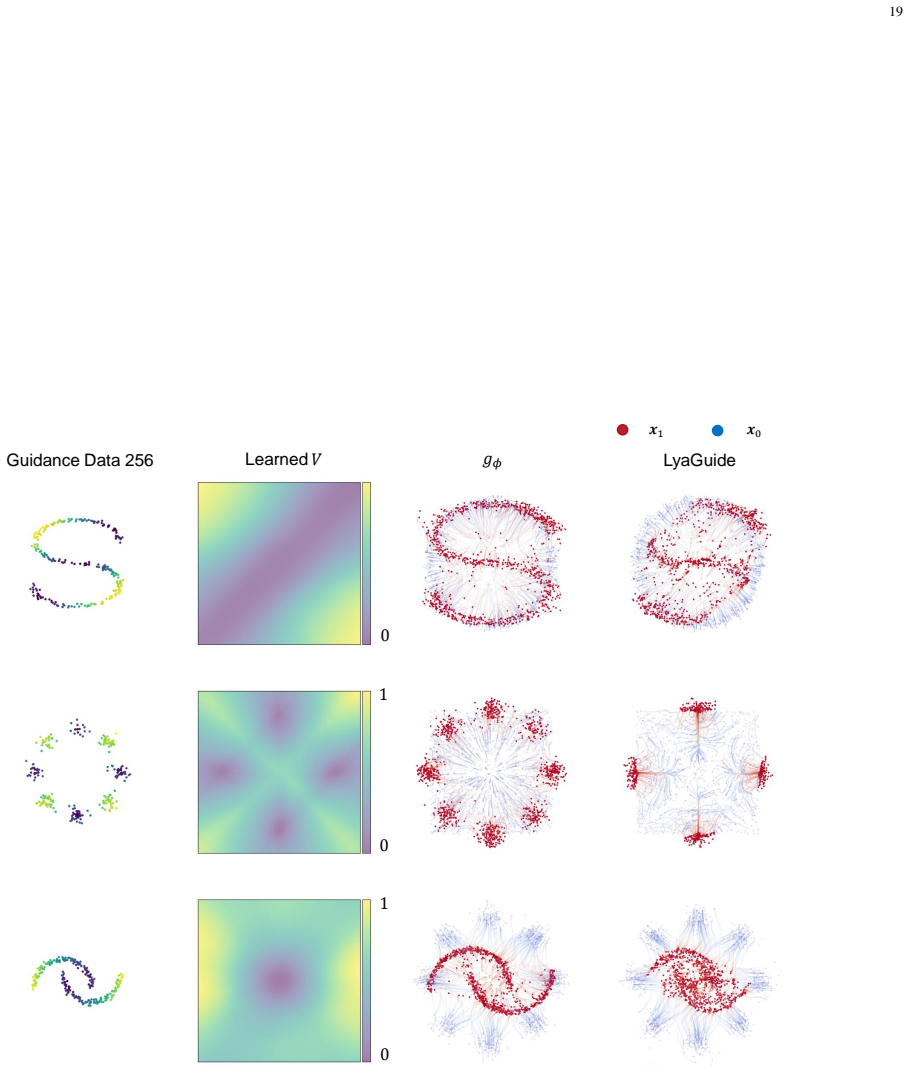
- In the data-driven setting, a learned Lyapunov function from few-shot preference–score pairs supplies the potential V, extending stability guarantees to tasks without analytic energy functions.
- Lyapunov-induced contraction accelerates convergence; the paper's early-inference-termination experiments show guided trajectories approach the target distribution substantially faster than their unguided counterparts.
- The framework unifies common guidance strategies as instances of Lyapunov control, giving a shared stability criterion and a common mathematical language for analyzing guidance in generative flows.
Where Pith is reading between the lines
- If the equivalence is taken as a design principle, other certificate functions from control theory—barrier functions or contraction metrics—could yield analogous closed-form corrections for generative flows, extending the stabilization idea beyond Lyapunov functions.
- Because the paper notes the pseudo-projection does not preserve the weighted continuity equation in general, a direct numerical check is to measure the residual of that equation after projection on a closed-form Gaussian example; small residuals would indicate conditional fidelity holds in practice despite the missing general guarantee.
- The exponential-initialization robustness result suggests LyaGuide could be combined with solvers whose starting distribution differs from the theoretical conditional prior, since the mismatch decays at rate e^{−δt}; this is a testable plug-in prediction for inverse-problem pipelines.
- The paper's Proposition 2 assigns the EBM Lyapunov function V = −E, while the appendix proof of the same claim takes V = E; since the Lyapunov decrease condition is sign-sensitive, aligning this convention is a concrete prerequisite before applying the pseudo-projection to EBM guidance.
Editorial analysis
A structured set of objections, weighed in public.
Referee Report
Summary. The paper proposes LyaGuide, a framework that reinterprets post-training guidance for flow-matching generative models as Lyapunov control. The central theoretical claim (Theorem 2) is an equivalence between guidance that samples a reweighted distribution p'_t = (1/Z_t)p_t e^{-J} and controllers satisfying a local Lyapunov condition with V related to J. The paper then introduces a closed-form 'pseudo-projection' (Theorem 3) that modifies any candidate guidance to enforce the Lyapunov inequality, and claims this can be applied to existing guidance methods without retraining while preserving conditional-sampling behavior. Two settings are considered: a model-driven setting with an explicit Lyapunov function and a data-driven setting where V is learned from few-shot data. Experiments cover synthetic 2D benchmarks, CelebA-HQ image inverse problems, D4RL offline RL planning, and energy matching.
Significance. If the claimed equivalence and projection guarantees were correct, the paper would provide a useful unification: any existing flow-guidance method could be stabilized by a simple pointwise correction at negligible cost. The paper is clearly written, includes extensive experiments with baseline comparisons, and makes a genuine attempt to connect control theory to generative modeling. However, the theoretical core is not sound as stated. The paper's own Discussion VI-a concedes that the pseudo-projection does not preserve the weighted continuity equation, so the projected field is not shown to generate the targeted conditional distribution. In addition, the sign of the Lyapunov function V is inconsistent between propositions and proofs, and the claimed contraction-based robustness result (Theorem 6) does not follow from the Lyapunov condition. These are load-bearing issues that invalidate the central claims.
major comments (5)
- [§VI-a, Theorem 3, Eq. (12)] The pseudo-projection in Theorem 3 enforces only the pointwise Lyapunov inequality. It does not enforce the weighted continuity equation (12) that is necessary for u_t + π(c_t) to generate p'_t = (1/Z_t)p_t e^{-J}. Section VI-a explicitly states that the projection 'does not preserve the weighted continuity equation in general.' Thus Theorem 3 proves membership in U_s only, not in U_g ∩ U_s, and Algorithm 1's output is not shown to perform conditional sampling. This directly contradicts the abstract and contributions, which claim that LyaGuide provides stability guarantees while remaining compatible with flow guidance.
- [Proposition 2 vs. Appendix B-C; Theorem 2 statement vs. proof Step 2] The sign convention for V is inconsistent. Proposition 2 states that for EBM guidance the Lyapunov function is V(x) = -E(x), while the proof in Appendix B-C says 'Interpreting V(x) = E(x) as Lyapunov function.' Similarly, Theorem 2 states V = J, but Step 2 of its proof constructs a Lyapunov-compatible control with V = -J. Since the Lyapunov inequality and the projection operator depend on the sign of V, these two conventions yield opposite descent directions. For a target density proportional to e^{-E}, taking V = -E makes low-energy modes maxima of V, so the Lyapunov condition would repel from, not attract to, the desired modes.
- [Theorem 6, Lemma 1, Eq. (22)] Theorem 6 claims that if the guided field satisfies the local Lyapunov condition with rate δ > 0, then W2(pt, p⋆_t) ≤ e^{-δt} W2(p0, p⋆_0). This does not follow from the Lyapunov inequality. The proof relies on the one-sided Lipschitz contractivity assumption (22), which is not implied by ∇V·(u+c) ≤ -δV. Lemma 1 introduces additional strong-convexity and operator-norm conditions (A1–A4) that are absent from the theorem statement. As stated, Theorem 6 is false in general, and the claimed robustness to the choice of initial distribution is unsupported.
- [Theorem 2, Appendix B-B] The theorem is titled 'Equivalence between Guided Flow Matching and Lyapunov Control,' but the proof only shows existence of a control lying in U_g ∩ U_s. It does not show that every guidance-compatible control satisfies the Lyapunov condition, nor that every Lyapunov-stable control is guidance-compatible. The construction of the tangential component c⊤_t in Step 2 also asserts solvability of the residual divergence equation under a tangency constraint based only on a zero-integral condition; this is not a sufficient condition for the existence of a tangential solution. The 'equivalence' claim is therefore an overstatement.
- [Theorem 3, Proposition 1] The pseudo-projection formula divides by ||∇V(x)||². At local minima of V, which are exactly the attractors in the multi-attractor setting of Proposition 1, ∇V = 0 and the projection is undefined. The paper states that π is locally Lipschitz, but this requires a uniform lower bound on ||∇V||, which is incompatible with having multiple isolated local minima. This technical gap affects the well-posedness of the guided flow near the target modes.
minor comments (5)
- [Equation (3)] The soft importance weight w_i = exp(-α V_i)/Σ exp(-α V_j) depends on the scale of V, and α is introduced without guidance on how to set it. Please discuss the sensitivity to α and the calibration of V.
- [Table II] In the box-inpainting experiments, LyaGuide-ES worsens FID for OT-CFM gMC (24.1950 vs 18.6635) and for CFM gcov-G (24.3271 vs 19.8022), while LyaGuide-CS improves them. The claim of 'consistent improvements' should be qualified, and the differing behavior of ES and CS variants explained.
- [Appendix B-E] The notation LyaGuide-ES, -AS, and -CS is used before the variants are formally defined in Section IV-A; consider defining them earlier or in a table.
- [General] Several references are to the authors' own prior work (e.g., [18], [19], [20], [54]) used to support claims of practical efficacy of jointly learned V and c. Please clarify the novelty relative to these works.
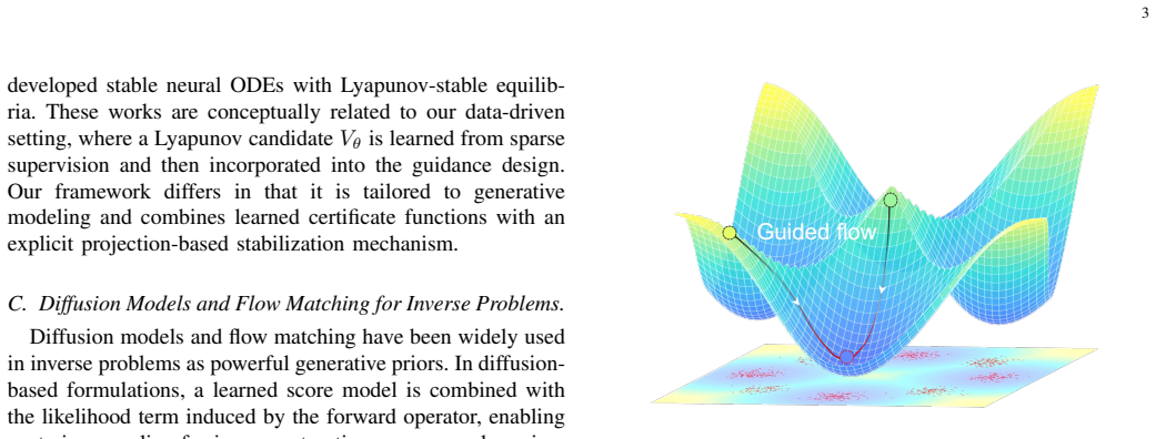
- [Figure 2] The figure illustrates the pseudo-projection but does not indicate that the result may leave the guidance-compatible set U_g. A remark pointing to the limitation stated in VI-a would help avoid confusion.
Circularity Check
No significant circularity: the pseudo-projection is an explicit construction and the self-citations are background; the main weakness is an unsupported conditional-sampling claim, not a circular derivation.
full rationale
The central derivation is not circular. Theorem 2 derives the weighted continuity equation (Eq. 12) from the definition of the reweighted path p'_t and constructs controls satisfying both the divergence constraint and the Lyapunov inequality via a normal/tangential decomposition; the reverse direction requires solving coupled PDEs (15)-(16), which is a substantive existence claim rather than a restatement of inputs. Theorem 3's pseudo-projection is defined as subtracting the positive part of the Lyapunov residual, so membership in U(V) holds by construction, but this is an explicit projection construction, not a fitted parameter renamed as a prediction. The paper does overstate the consequence: Section IV-B claims 'theoretical guarantees of conditional sampling via Lyapunov stability,' while Section VI-a concedes 'the projection ... does not preserve the weighted continuity equation in general,' so Algorithm 1 only enforces Lyapunov decrease, not sampling from p'_t; this is a correctness gap, not circularity. Self-citations [18], [19], [20], [54] appear as background related-work and joint-training mentions, not as load-bearing support for the equivalence or the projection. The EBM sign inconsistency (V=-E in Proposition 2 vs V=E in the Appendix B-C proof) is an internal inconsistency, not a circular step. No fitted values are disguised as predictions; experiments compare baseline guidance with and without LyaGuide under identical settings.
Axiom & Free-Parameter Ledger
free parameters (4)
- δ (Lyapunov decay rate / projection strength) =
0.2–2.0 ablated; recommendation δ ∈ [0,1]
- k (gradient-based candidate guidance strength) =
0.5–1.5 ablated
- α (soft importance weight temperature in Eq. (3)) =
not reported
- Parameters of learned Lyapunov V_θ =
3-layer MLP, width 64, weighted regression
axioms (5)
- domain assumption Base flow satisfies the continuity equation ∂_t p_t + ∇·(p_t u_t)=0 with vanishing boundary terms at infinity or periodic boundaries.
- ad hoc to paper For any RHS with zero integral, the divergence equation ∇·(p'_t c_t)=RHS admits solutions, and a tangential component can be chosen to satisfy the residual.
- domain assumption The target conditional distribution is exactly p'_t=(1/Z_t)p_t e^{-J(x)} with time-independent J.
- domain assumption V is sufficiently smooth and ∇V ≠ 0 along trajectories so the pseudo-projection is well-defined.
- domain assumption V has the sign convention such that decreasing V moves toward high-probability regions of the guided distribution.
read the original abstract
Flow matching has emerged as an effective framework for learning complex data distributions, but adapting pretrained flow models to new tasks often requires computationally expensive retraining. Post-training guidance provides a more efficient alternative, but existing methods are largely heuristic and offer no explicit stability guarantees. We address this limitation by proposing LyaGuide, a unified Lyapunov-guided framework that formulates flow guidance as a Lyapunov control problem. Our main theoretical result establishes an equivalence between guided flow matching and Lyapunov control, thereby unifying common guidance strategies, such as classifier guidance, reward guidance, and energy-based guidance, within a single control-theoretic framework. To enforce the Lyapunov condition, we introduce a pseudo-projection operator with a closed-form expression that endows learned or heuristic guidance terms with explicit stability guarantees. LyaGuide supports two practical settings: a model-driven setting, where the target guidance distribution is specified through a known Lyapunov function, and a data-driven setting, where the guidance is adapted from task-specific downstream data. LyaGuide is compatible with existing guidance methods, introduces minimal additional computational overhead, and is straightforward to integrate in practice. Extensive experiments on synthetic benchmarks, image inverse problems, reinforcement learning planning, and energy-based modeling demonstrate consistent improvements in sample quality, guidance fidelity, and robustness, while maintaining computational efficiency.
Figures




Reference graph
Works this paper leans on
-
[1]
Score-based generative modeling through stochastic differ- ential equations,
Y . Song, J. Sohl-Dickstein, D. P. Kingma, A. Kumar, S. Ermon, and B. Poole, “Score-based generative modeling through stochastic differ- ential equations,” inInternational Conference on Learning Representa- tions, 2021
2021
-
[2]
Diffusion models beat gans on image synthesis,
P. Dhariwal and A. Nichol, “Diffusion models beat gans on image synthesis,”Advances in neural information processing systems, vol. 34, pp. 8780–8794, 2021
2021
-
[3]
Classifier-free diffusion guidance,
J. Ho and T. Salimans, “Classifier-free diffusion guidance,” inNeurIPS 2021 Workshop on Deep Generative Models and Downstream Applica- tions
2021
-
[4]
Flow matching for generative modeling,
Y . Lipman, R. T. Chen, H. Ben-Hamu, M. Nickel, and M. Le, “Flow matching for generative modeling,” in11th International Conference on Learning Representations, ICLR 2023, 2023
2023
-
[5]
Flow straight and fast: Learning to generate and transfer data with rectified flow,
X. Liu, C. Gonget al., “Flow straight and fast: Learning to generate and transfer data with rectified flow,” inThe Eleventh International Conference on Learning Representations, 2023
2023
-
[6]
Conditional flow matching: Simulation-free dynamic optimal transport,
A. Tong, N. Malkin, G. Huguet, Y . Zhang, J. Rector-Brooks, K. Fatras, G. Wolf, and Y . Bengio, “Conditional flow matching: Simulation-free dynamic optimal transport,”arXiv preprint arXiv:2302.00482, vol. 2, no. 3, 2023
Pith/arXiv arXiv 2023
-
[7]
Cfg-zero*: Improved classifier-free guidance for flow matching models,
W. Fan, A. Y . Zheng, R. A. Yeh, and Z. Liu, “Cfg-zero*: Improved classifier-free guidance for flow matching models,”CoRR, 2025
2025
-
[8]
On the guidance of flow matching,
R. Feng, C. Yu, W. Deng, P. Hu, and T. Wu, “On the guidance of flow matching,” inForty-second International Conference on Machine Learning, 2025
2025
-
[9]
Generalized protein pocket generation with prior-informed flow matching,
Z. Zhang, M. Zitnik, and Q. Liu, “Generalized protein pocket generation with prior-informed flow matching,”Advances in neural information processing systems, vol. 37, pp. 38 559–38 589, 2024
2024
-
[10]
Planning with diffusion for flexible behavior synthesis,
M. Janner, Y . Du, J. Tenenbaum, and S. Levine, “Planning with diffusion for flexible behavior synthesis,” inInternational Conference on Machine Learning. PMLR, 2022, pp. 9902–9915
2022
-
[11]
Solving inverse problems in medical imaging with score-based generative models,
Y . Song, L. Shen, L. Xing, and S. Ermon, “Solving inverse problems in medical imaging with score-based generative models,”arXiv preprint arXiv:2111.08005, 2021
Pith/arXiv arXiv 2021
-
[12]
Denoising diffusion restoration models,
B. Kawar, M. Elad, S. Ermon, and J. Song, “Denoising diffusion restoration models,”Advances in neural information processing systems, vol. 35, pp. 23 593–23 606, 2022
2022
-
[13]
Diffusion posterior sampling for general noisy inverse problems,
H. Chung, J. Kim, M. T. Mccann, M. L. Klasky, and J. C. Ye, “Diffusion posterior sampling for general noisy inverse problems,” inThe Eleventh International Conference on Learning Representations
-
[14]
Nonlinear systems third edition,
H. K. Khalil, “Nonlinear systems third edition,”Patience Hall, vol. 115, 2002
2002
-
[15]
P. A. Parrilo,Structured Semidefinite Programs and Semialgebraic Geometry Methods in Robustness and Optimization. California Institute of Technology, 2000
2000
-
[16]
Contraction theory for nonlinear stability analysis and learning-based control: A tutorial overview,
H. Tsukamoto, S.-J. Chung, and J.-J. E. Slotine, “Contraction theory for nonlinear stability analysis and learning-based control: A tutorial overview,”Annual Reviews in Control, vol. 52, pp. 135–169, 2021
2021
-
[17]
Neural lyapunov control,
Y .-C. Chang, N. Roohi, and S. Gao, “Neural lyapunov control,” in Proceedings of the 33rd International Conference on Neural Information Processing Systems, 2019, pp. 3245–3254
2019
-
[18]
Neural stochastic control,
J. Zhang, Q. Zhu, and W. Lin, “Neural stochastic control,” inAdvances in Neural Information Processing Systems, 2022
2022
-
[19]
Neural event-triggered control with optimal scheduling,
L. Yang, J. Zhang, Q. Zhu, and W. Lin, “Neural event-triggered control with optimal scheduling,”arXiv preprint arXiv:2507.14653, 2025
Pith/arXiv arXiv 2025
-
[20]
Sync: Safety-aware neural control for stabilizing stochastic delay-differential equations,
J. Zhang, Q. Zhu, W. Yang, and W. Lin, “Sync: Safety-aware neural control for stabilizing stochastic delay-differential equations,” inThe Eleventh International Conference on Learning Representations, 2022
2022
-
[21]
Learning safe multi-agent control with decentralized neural barrier certificates,
Z. Qin, K. Zhang, Y . Chen, J. Chen, and C. Fan, “Learning safe multi-agent control with decentralized neural barrier certificates,” in International Conference on Learning Representations, 2020
2020
-
[22]
Learning certified control using contraction metric,
D. Sun, S. Jha, and C. Fan, “Learning certified control using contraction metric,” inConference on Robot Learning. PMLR, 2021, pp. 1519– 1539
2021
-
[23]
Stabilization with relaxed controls,
Z. Artstein, “Stabilization with relaxed controls,”Nonlinear Analysis: Theory, Methods & Applications, vol. 7, no. 11, pp. 1163–1173, 1983
1983
-
[24]
A ‘universal’construction of artstein’s theorem on nonlin- ear stabilization,
E. D. Sontag, “A ‘universal’construction of artstein’s theorem on nonlin- ear stabilization,”Systems & control letters, vol. 13, no. 2, pp. 117–123, 1989
1989
-
[25]
Nonlinear feedback design for fixed-time stabilization of linear control systems,
A. Polyakov, “Nonlinear feedback design for fixed-time stabilization of linear control systems,”IEEE Transactions on Automatic Control, vol. 57, no. 8, pp. 2106–2110, 2012
2012
-
[26]
Calibrated multi-preference optimization for align- ing diffusion models,
K. Lee, X. Li, Q. Wang, J. He, J. Ke, M.-H. Yang, I. Essa, J. Shin, F. Yang, and Y . Li, “Calibrated multi-preference optimization for align- ing diffusion models,” inProceedings of the Computer Vision and Pattern Recognition Conference, 2025, pp. 18 465–18 475
2025
-
[27]
Training diffu- sion models with reinforcement learning,
K. Black, M. Janner, Y . Du, I. Kostrikov, and S. Levine, “Training diffu- sion models with reinforcement learning,” inThe Twelfth International Conference on Learning Representations, 2023
2023
-
[28]
Towards controllable diffusion models via reward- guided exploration,
H. Zhang and T. Xu, “Towards controllable diffusion models via reward- guided exploration,”arXiv preprint arXiv:2304.07132, 2023
Pith/arXiv arXiv 2023
-
[29]
A tutorial on energy-based learning,
Y . LeCun, S. Chopra, R. Hadsell, M. Ranzato, F. Huanget al., “A tutorial on energy-based learning,”Predicting structured data, vol. 1, no. 0, 2006
2006
-
[30]
Incorporating stability into flow matching,
C. I. Sprague, A. Elofsson, and H. Azizpour, “Incorporating stability into flow matching,” inICML 2024 Workshop on Structured Probabilistic Inference{\&}Generative Modeling, 2024
2024
-
[31]
Stochastic interpolant: A new framework for generative modeling,
M. S. Albergo, M. Rizzi, and K. Cranmer, “Stochastic interpolant: A new framework for generative modeling,” inInternational Conference on Machine Learning (ICML), 2023
2023
-
[32]
Generative modeling with phase stochas- tic bridges,
T. Chen, J. Gu, and L. Dinh, “Generative modeling with phase stochas- tic bridges,” inInternational Conference on Learning Representations (ICLR), 2023
2023
-
[33]
Generative modeling by estimating gradients of the data distribution,
Y . Song and S. Ermon, “Generative modeling by estimating gradients of the data distribution,”Advances in neural information processing systems, vol. 32, 2019
2019
-
[34]
Implicit generation and modeling with energy based models,
Y . Du and I. Mordatch, “Implicit generation and modeling with energy based models,”Advances in neural information processing systems, vol. 32, 2019
2019
-
[35]
Physics-informed neural network lyapunov functions: Pde characterization, learning, and verification,
J. Liu, Y . Meng, and M. Fitzsimmons, “Physics-informed neural network lyapunov functions: Pde characterization, learning, and verification,” Journal of Machine Learning Research, vol. 24, no. 210, pp. 1–36, 2023
2023
-
[36]
Stable neural ode with lyapunov-stable equilibrium points for defending against adversarial attacks,
Q. Kang, Y . Song, Q. Ding, and W. P. Tay, “Stable neural ode with lyapunov-stable equilibrium points for defending against adversarial attacks,”Advances in Neural Information Processing Systems, vol. 34, pp. 14 925–14 937, 2021
2021
-
[37]
Zero-shot image restoration using denoising diffusion null-space model,
Y . Wang, J. Yu, and J. Zhang, “Zero-shot image restoration using denoising diffusion null-space model,” inThe Eleventh International Conference on Learning Representations
-
[38]
Pseudoinverse-guided diffusion models for inverse problems,
J. Song, A. Vahdat, M. Mardani, and J. Kautz, “Pseudoinverse-guided diffusion models for inverse problems,” inInternational Conference on Learning Representations, 2023
2023
-
[39]
Training-free linear image inverses via flows,
A. Pokle, M. J. Muckley, R. T. Chen, and B. Karrer, “Training-free linear image inverses via flows,”arXiv preprint arXiv:2310.04432, 2023
Pith/arXiv arXiv 2023
-
[40]
Flow priors for linear inverse problems via iterative corrupted trajectory matching,
Y . Zhang, P. Yu, Y . Zhu, Y . Chang, F. Gao, Y . N. Wu, and O. Leong, “Flow priors for linear inverse problems via iterative corrupted trajectory matching,”Advances in Neural Information Processing Systems, vol. 37, pp. 57 389–57 417, 2024
2024
-
[41]
Pnp-flow: Plug- and-play image restoration with flow matching,
S. Martin, A. Gagneux, P. Hagemann, and G. Steidl, “Pnp-flow: Plug- and-play image restoration with flow matching,” inInternational Con- ference on Learning Representations, 2025
2025
-
[42]
Fig: Flow with interpolant guidance for linear inverse problems,
Y . Yan, Y . Zhang, X. Meng, and Z. Zhao, “Fig: Flow with interpolant guidance for linear inverse problems,” inThe Thirteenth International Conference on Learning Representations, 2025
2025
-
[43]
Film: Visual reasoning with a general conditioning layer,
E. Perez, F. Strub, H. De Vries, V . Dumoulin, and A. Courville, “Film: Visual reasoning with a general conditioning layer,” inProceedings of the AAAI conference on artificial intelligence, vol. 32, no. 1, 2018
2018
-
[44]
Learning multiple visual domains with residual adapters,
S.-A. Rebuffi, H. Bilen, and A. Vedaldi, “Learning multiple visual domains with residual adapters,” inNeurIPS, 2017
2017
-
[45]
Efficient parametrization of multi-domain deep neural networks,
——, “Efficient parametrization of multi-domain deep neural networks,” inProceedings of the IEEE conference on computer vision and pattern recognition, 2018, pp. 8119–8127
2018
-
[46]
Model-agnostic meta-learning for fast adaptation of deep networks,
C. Finn, P. Abbeel, and S. Levine, “Model-agnostic meta-learning for fast adaptation of deep networks,” inICML, 2017
2017
-
[47]
Meta-learning with latent embedding optimization,
A. A. Rusu, D. Rao, J. Sygnowski, R. Pascanu, S. Osindero, and R. Hadsell, “Meta-learning with latent embedding optimization,” in ICLR, 2019
2019
-
[48]
Parameter-efficient transfer learning for nlp,
N. Houlsby, A. Giurgiu, S. Jastrzebski, B. Morrone, Q. De Laroussilhe, A. Gesmundo, M. Attariyan, and S. Gelly, “Parameter-efficient transfer learning for nlp,” inInternational conference on machine learning. PMLR, 2019, pp. 2790–2799
2019
-
[49]
Wiener,Cybernetics or Control and Communication in the Animal and the Machine
N. Wiener,Cybernetics or Control and Communication in the Animal and the Machine. MIT press, 2019
2019
-
[50]
Mao,Stochastic differential equations and applications
X. Mao,Stochastic differential equations and applications. Elsevier, 2007
2007
-
[51]
Safe control with learned certificates: A survey of neural lyapunov, barrier, and contraction methods for robotics and control,
C. Dawson, S. Gao, and C. Fan, “Safe control with learned certificates: A survey of neural lyapunov, barrier, and contraction methods for robotics and control,”IEEE Transactions on Robotics, 2023. 25
2023
-
[52]
Projection-based integrators for improved motion control: Formalization, well-posedness and stability of hybrid integrator- gain systems,
D. A. Deenen, B. Sharif, S. van den Eijnden, H. Nijmeijer, M. Heemels, and M. Heertjes, “Projection-based integrators for improved motion control: Formalization, well-posedness and stability of hybrid integrator- gain systems,”Automatica, vol. 133, p. 109830, 2021
2021
-
[53]
Lyapunov-based safe policy optimization for continuous control,
Y . Chow, O. Nachum, A. Faust, E. Duenez-Guzman, and M. Ghavamzadeh, “Lyapunov-based safe policy optimization for continuous control,”arXiv preprint arXiv:1901.10031, 2019
Pith/arXiv arXiv 1901
-
[54]
Fessnc: Fast exponentially sta- ble and safe neural controller,
J. Zhang, L. Yang, Q. Zhu, and W. Lin, “Fessnc: Fast exponentially sta- ble and safe neural controller,” inInternational Conference on Machine Learning. PMLR, 2024, pp. 60 076–60 098
2024
-
[55]
Contrastive energy prediction for exact energy-guided diffusion sampling in offline rein- forcement learning,
C. Lu, H. Chen, J. Chen, H. Su, C. Li, and J. Zhu, “Contrastive energy prediction for exact energy-guided diffusion sampling in offline rein- forcement learning,” inInternational Conference on Machine Learning. PMLR, 2023, pp. 22 825–22 855
2023
-
[56]
D4rl: Datasets for deep data-driven reinforcement learning,
J. Fu, A. Kumar, O. Nachum, G. Tucker, and S. Levine, “D4rl: Datasets for deep data-driven reinforcement learning,”arXiv preprint arXiv:2004.07219, 2020
Pith/arXiv arXiv 2004
-
[57]
Flow matching on general geometries,
R. T. Chen and Y . Lipman, “Flow matching on general geometries,” in 12th International Conference on Learning Representations, ICLR 2024, 2024
2024
-
[58]
Reinforcement learning and control as probabilistic infer- ence: Tutorial and review,
S. Levine, “Reinforcement learning and control as probabilistic infer- ence: Tutorial and review,”arXiv preprint arXiv:1805.00909, 2018
Pith/arXiv arXiv 2018
-
[59]
Energy matching: Unifying flow matching and energy-based models for generative mod- eling,
M. Balcerak, T. Amiranashvili, A. Terpin, S. Shit, L. Bogensperger, S. Kaltenbach, P. Koumoutsakos, and B. Menze, “Energy matching: Unifying flow matching and energy-based models for generative mod- eling,” inThe Thirty-ninth Annual Conference on Neural Information Processing Systems, 2025
2025
-
[60]
Finite-time and fixed-time stabilization: Implicit lyapunov function approach,
A. Polyakov, D. Efimov, and W. Perruquetti, “Finite-time and fixed-time stabilization: Implicit lyapunov function approach,”Automatica, vol. 51, pp. 332–340, 2015
2015
discussion (0)
Sign in with ORCID, Apple, or X to comment. Anyone can read and Pith papers without signing in.