REVIEW 3 major objections 6 minor 34 references
Sequentially adapting SAM to alloy microstructures before XCT defect data improves pore and inclusion segmentation with only 4.15M trainable parameters.
Reviewed by Pith at T0; open to challenge. T0 means a machine referee read the full paper against a public rubric. the ladder, T0–T4 →
T0 review · deepseek-v4-flash
2026-08-02 02:31 UTC pith:JOJKJIIL
load-bearing objection Useful empirical recipe, but the central causal claim about sequential bridging is not yet supported—the two-stage model gets extra training time and a different schedule than the direct baseline. the 3 major comments →
XCT-SAM: Sequential Parameter-Efficient Domain Adaptation of SAM for Industrial XCT Defect Segmentation
The pith
A machine-rendered reading of the paper's core claim, the machinery that carries it, and where it could break.
Core claim
On its own terms, the paper establishes that a curriculum-like sequential adaptation of SAM's frozen image encoder—first on real alloy-microstructure images, then on synthetic XCT defect images—produces better out-of-distribution defect segmentation than adapting on XCT alone. The gains are attributed to the intermediate stage warming up the low-rank adapter weights toward metallic, low-contrast spatial features, so the limited XCT labels drive a smaller domain shift. Measured on IoU, Dice, and F1 across six synthetic test sets and multiple real-world scan sets, the best configuration (rank 2, eight convolutional experts, Dice-Focal loss) outperforms every baseline on both pore and inclusion
What carries the argument
Conv-LoRA, a parameter-efficient adapter that injects a low-rank update plus a set of convolutional expert gates into each transformer block of SAM's frozen ViT-H encoder. The adapter computes an embedding update of the form W0x + WD(Σ gi(x) Ei(WEx)), where WE and WD are low-rank projections, Ei are convolutional experts, and gi are gating weights. XCT-SAM's central use of this mechanism is sequential: the adapter weights are first trained for up to 15 epochs on alloy-microstructure images, then re-trained with a lower learning rate for 20 more epochs on GAN-generated XCT images. The paper argues that this warm start decomposes the large natural-image-to-XCT shift into two smaller shifts.
Load-bearing premise
The claim that the intermediate alloy training stage—rather than the extra training time or different optimization schedule it introduces—is what drives the performance improvement is not directly tested, because the direct baseline receives fewer total training updates.
What would settle it
Train the direct Conv-LoRA-SAM baseline on the same XCT data for exactly the combined number of epochs (15 alloy + 20 XCT) with the same two-stage learning-rate schedule, except skip the alloy stage and either keep the same total steps or use the first 15 epochs on XCT data. If this matched-cost baseline matches or exceeds XCT-SAM's IoU/Dice on the synthetic and real test sets, the sequential-bridging claim fails.
If this is right
- If the sequential adaptation claim holds, SAM-based industrial XCT defect segmentation becomes practical on small labeled datasets, with most of the model frozen.
- The intermediate-domain warm-start recipe could be reused for other non-destructive-testing modalities where labeled defect data are scarce but related material-imaging data exist.
- The rank-2 result suggests that very low-rank adapters are sufficient for sparse, low-contrast defect domains, and that higher ranks can hurt rare-class generalization.
- The loss-function study indicates that Dice-Focal is a robust default for extreme class imbalance, outperforming plain Dice, BCE, Lovász-Softmax, and Focal Tversky on the tested benchmarks.
Where Pith is reading between the lines
- The paper does not rule out that the alloy stage simply provides extra training time or a favorable learning-rate schedule; a matched step-count control without the alloy stage would be needed to isolate the bridging effect.
- The approach may extend to 3D volumetric segmentation by slotting the same two-stage adapter schedule into a volumetric SAM variant, though the paper tests only 2D slices.
- Because the real-world reference masks are threshold-derived, part of the reported real-world gain could reflect alignment with the thresholding pipeline rather than with true defect geometry; ground-truth labels from human annotation or higher-resolution scans would be a stronger test.
- The two independent binary models create redundant computation; a unified multiclass model with a class-balanced loss might reach similar accuracy at lower inference cost.
Editorial analysis
A structured set of objections, weighed in public.
Referee Report
Summary. The paper proposes XCT-SAM, a two-stage parameter-efficient domain adaptation method for SAM-based defect segmentation in additive-manufacturing XCT images. In Stage 1, Conv-LoRA adapters (rank r=2, eight convolutional experts) are fine-tuned on an alloy-microstructure dataset; in Stage 2, the adapters are further fine-tuned on CycleGAN-generated synthetic XCT data. The authors report evaluations on synthetic GAN-XCT benchmarks and real NIST XCT scans, comparing against zero-shot SAM, UNet++, MedSAM, SAM-Med2D, and direct Conv-LoRA-SAM. They report the best overall IoU and Dice across all settings with 4.15M trainable parameters (0.647% of the model), and release the code.
Significance. If the two-stage bridging claim is supported, the contribution is practically useful: it combines an intermediate material-domain adaptation stage with parameter-efficient Conv-LoRA to improve SAM on sparse, non-semantic industrial defects, and includes evaluations on an external real-world NIST dataset. Strengths include the public code release, the consideration of real XCT data, and ablations over rank and loss objectives. The main reservation is that the central attribution — that the intermediate alloy stage, not extra training compute or a different schedule, drives the gains — is not directly tested because no matched-compute direct baseline is included.
major comments (3)
- [Sec. IV-B and IV-D, Table I] The central claim that the alloy intermediate stage causes the reported gains is not isolated from training compute and schedule. XCT-SAM is trained for 15 alloy epochs at LR 2e-4 plus 20 XCT epochs at LR 8e-5 (Sec. IV-D), while the direct Conv-LoRA-SAM baseline is described only as fine-tuned on GAN XCT without the alloy stage (Sec. IV-B); its epoch count, total updates, and LR schedule are not reported. If the baseline is trained only for the Stage-2 budget, the +0.0472 IoU (pores) and +0.1232 IoU (inclusions) margins in Table I could come from longer training, the higher initial LR, or warm-start initialization rather than from the alloy domain specifically. The ablation study in Tables II–III also never removes Stage 1 while holding compute fixed. I request a matched-compute control: train direct Conv-LoRA-SAM on XCT for the same total number of updates and with the same LR schedule
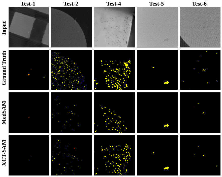
- [Sec. IV-A and Table I] The evaluation protocol appears to include the validation set in the reported averages. Section IV-A states that Test-3 is used as the validation set because it clusters closely with Train-1 and Train-2, but Table I reports means computed 'across all test sets,' and the quantitative text in Sec. IV-E refers to 'all test sets' without excluding Test-3. Including the validation set in final averaged numbers can inflate reported performance and makes the benchmark less clean. Please report per-test-set results and recalculate the averages either excluding Test-3 or explicitly treating it as a held-out validation set with no hyperparameter selection.
- [Sec. IV-A, NIST evaluation] The NIST ground-truth masks are not publicly available, so the authors generate threshold-derived reference masks following the pipeline of [33]. This means the NIST results evaluate agreement with a threshold-based proxy rather than with expert annotations. The threshold value and preprocessing steps are not reported, and no sensitivity analysis is provided. Since the NIST benchmark is a major part of the claim of real-world generalization, the threshold-dependence of the reference masks should be quantified (e.g., report performance over a range of thresholds or compare against any available published segmentations). Without this, the NIST IoU/Dice numbers are difficult to interpret and reproduce.
minor comments (6)
- [Fig. 4] The t-SNE analysis uses ViT-B/16 features, but the adapted model uses a ViT-H encoder. Please clarify whether the ViT-B/16 features are from the original SAM, from a Conv-LoRA-adapted model, and why this feature space is representative of the ViT-H backbone used in all experiments.
- [Eq. (1)] The gating function and convolutional expert details are not fully specified. Please define the gating network, the kernel sizes/strides of the convolutional experts, and how the number of experts (eight) is chosen; this would also make the rank/parameter-count ablation in Table II more reproducible.
- [Table I and Fig. 5] Table I reports only mean values without variance or statistical significance. Fig. 5 shows error bars, but the number of runs/seeds and the source of the variance are not stated in the table or text. Reporting per-test-set values or standard deviations in the table would make the margins between XCT-SAM and Conv-LoRA-SAM more interpretable.
- [Table III] The F1 column appears to be the tolerance-based F1 defined in Sec. IV-C, but the table header uses 'F1' without the qualifier. Please rename it to 'Tolerance-F1' for consistency and to avoid confusion with the Dice coefficient.
- [Sec. IV-F] The ablation studies vary rank and loss but do not vary the number of convolutional experts, although the abstract and conclusion highlight 'eight convolutional experts' as part of the best configuration. A brief sentence justifying this fixed value or an ablation over the number of experts would strengthen the parameter-efficiency analysis.
- [Sec. V] The limitations paragraph mentions the additional cost of two-stage training but does not report the actual compute overhead (epochs, GPU-hours, or wall-clock time) relative to direct Conv-LoRA-SAM. Please include a quantitative comparison of training cost.
Circularity Check
No significant circularity: the central claim is an empirical comparison against external benchmarks.
full rationale
The paper's central claim is that a two-stage adaptation (alloy-microstructure then XCT) improves SAM-based defect segmentation. This is established empirically by training XCT-SAM and comparing its IoU/Dice/F1 on held-out CycleGAN-XCT test sets and independent real NIST XCT scans against several baselines. There is no mathematical derivation in which a predicted quantity reduces to a fitted constant by construction. The Conv-LoRA update equation (Sec. III-A) and the loss choices (Sec. III-B) contain no test-set statistics, and the reported metrics are not solved for from the training data. The alloy intermediate stage is a training schedule choice, not a self-definitional trick that guarantees the outcome. Self-citation is minimal and not load-bearing: reference [17] includes a co-author but is cited only as related work, while the main prior baseline [18] and the Conv-LoRA method [26] are external. The most serious weakness is the missing control for total training compute: no direct Conv-LoRA-SAM baseline is trained for the same number of epochs and learning-rate schedule as XCT-SAM, so the causal attribution of gains to the alloy stage is not fully isolated. That is a correctness/experimental-design risk, not circularity, and it does not make the reported results equivalent to the inputs. The paper is self-contained against external benchmarks, so the appropriate circularity score is 0.
Axiom & Free-Parameter Ledger
free parameters (8)
- Conv-LoRA rank r =
2
- Number of convolutional experts =
8
- Stage-I learning rate =
2e-4
- Stage-II learning rate =
8e-5
- Epochs (Stage-I, Stage-II) =
15, 20
- Batch size =
8
- Dice-Focal hyperparameters (alpha/gamma) =
unspecified
- NIST reference-mask threshold =
unspecified
axioms (4)
- domain assumption Alloy-microstructure images are an effective intermediate domain for AM XCT defects
- domain assumption CycleGAN-generated synthetic XCT images with preserved labels are a valid proxy for real XCT training data
- domain assumption Threshold-derived binary masks from NIST scans are a valid proxy for ground-truth defects
- domain assumption SAM's frozen ViT-H representations are a useful prior for this domain
read the original abstract
Defect segmentation in additive manufacturing (AM) X-ray computed tomography (XCT) images remains challenging due to severe class imbalance and large distribution shifts across scan conditions. Although recent foundation models such as the Segment Anything Model (SAM) provide strong general-purpose segmentation priors, their natural-image pre-training transfers poorly to the AM XCT domain, where defects appear as subtle non-semantic microstructural anomalies. Moreover, adapting SAM to the AM domain is further limited by the large domain gap and scarcity of labeled real XCT data. We present XCT-SAM, a sequential parameter-efficient adaptation framework for AM XCT defect segmentation. Instead of adapting SAM directly from natural images to XCT data, we first fine-tune Conv-LoRA adapters on an alloy-microstructure dataset and subsequently transfer the adapted model to XCT images, progressively bridging the domain gap. Using Conv-LoRA adapters with rank r=2, the framework injects convolutional spatial inductive bias into SAM's backbone while training approximately 4.15M parameters and keeping over 99% of the model frozen. We evaluate XCT-SAM on out-of-distribution CycleGAN-XCT benchmarks and real-world NIST XCT scans. Across both settings, XCT-SAM consistently outperforms zero-shot SAM and other domain-adapted SAM baselines, achieving the best overall IoU and Dice scores. These results demonstrate the effectiveness of intermediate domain adaptation with parameter-efficient adapters for industrial XCT defect segmentation. The source code is publicly available at https://github.com/Mahedi-61/XCT-SAM.git
Figures



Reference graph
Works this paper leans on
-
[1]
Additive manufacturing (3d printing): A review of materials, methods, applications and challenges,
T. D. Ngo, A. Kashani, G. Imbalzano, K. T. Nguyen, and D. Hui, “Additive manufacturing (3d printing): A review of materials, methods, applications and challenges,”Composites Part B: Engineering, vol. 143, pp. 172–196, 2018
2018
-
[2]
Recent advances in metal additive manufacturing: Materials design and artificial intelligence applications,
S. Wang, L. Zhou, S. Zhong, G. Li, L. Zhang, X. Wang, Z. Li, and J. Lu, “Recent advances in metal additive manufacturing: Materials design and artificial intelligence applications,”Engineering, 2026
2026
-
[3]
Metal additive manufacturing in aerospace: A review,
B. Blakey-Milner, P. Gradl, G. Snedden, M. Brooks, J. Pitot, E. Lopez, M. Leary, F. Berto, and A. Du Plessis, “Metal additive manufacturing in aerospace: A review,”Materials & Design, vol. 209, p. 110008, 2021
2021
-
[4]
Comprehensive review of fabrication process parameters influencing defect formation in laser powder bed fused (l-pbf) al-si alloys,
M. M. H. Tusher and A. Ince, “Comprehensive review of fabrication process parameters influencing defect formation in laser powder bed fused (l-pbf) al-si alloys,”Materials & Design, p. 114374, 2025
2025
-
[5]
Defects in metal additive manu- facturing: formation, process parameters, postprocessing, challenges, economic aspects, and future research directions,
R. Haribaskar and T. S. Kumar, “Defects in metal additive manu- facturing: formation, process parameters, postprocessing, challenges, economic aspects, and future research directions,”3D Printing and Additive Manufacturing, vol. 11, no. 4, pp. 1629–1655, 2024
2024
-
[6]
Feature-based volumetric defect classification in metal additive manufacturing,
A. Poudel, M. S. Yasin, J. Ye, J. Liu, A. Vinel, S. Shao, and N. Sham- saei, “Feature-based volumetric defect classification in metal additive manufacturing,”Nature Communications, vol. 13, no. 1, p. 6369, 2022
2022
-
[7]
Porosity defects in additively manufactured metal materials: Formation mecha- nisms, impact on performance and regulation,
L. Wang, S. Feng, Y . Wang, X. Zhao, J. Ge, T. Gao, and F. Di, “Porosity defects in additively manufactured metal materials: Formation mecha- nisms, impact on performance and regulation,”International Materials Reviews, vol. 71, no. 2, pp. 97–128, 2026
2026
-
[8]
Assessment of the effect of the process-induced porosity defects on the fatigue properties of wire arc additive manufactured al– si–mg alloy,
T. Zhan, K. Xu, Z. Fan, H. Xiang, C. Xu, T. Mei, Y . Wei, W. Chen, and L. Li, “Assessment of the effect of the process-induced porosity defects on the fatigue properties of wire arc additive manufactured al– si–mg alloy,”Journal of Materials Research and Technology, vol. 35, pp. 777–791, 2025
2025
-
[9]
Rapid non-destructive inspec- tion of sub-surface defects in 3D printed alumina through 30 layers with 7µm depth resolution,
C. Lapre, D. Brouczek, M. Schwentenwein, K. Neumann, N. Benson, C. Petersen, O. Bang, and N. Israelsen, “Rapid non-destructive inspec- tion of sub-surface defects in 3D printed alumina through 30 layers with 7µm depth resolution,”Open Ceramics, vol. 18, p. 100611, 2024
2024
-
[10]
Detecting and classifying hidden defects in additively manufactured parts using deep learning and x-ray computed tomography,
M. V . Bimrose, T. Hu, D. J. McGregor, J. Wang, S. Tawfick, C. Shao, Z. Liu, and W. P. King, “Detecting and classifying hidden defects in additively manufactured parts using deep learning and x-ray computed tomography,”Journal of Intelligent Manufacturing, vol. 36, no. 5, pp. 3465–3479, 2025
2025
-
[11]
X-ray computed tomography in metal additive manufacturing: A review on pre- vention, diagnostic, and prediction of failure,
X. Sun, L. Huang, B. Xiao, Q. Zhang, J. Li, and Y . e. a. Ding, “X-ray computed tomography in metal additive manufacturing: A review on pre- vention, diagnostic, and prediction of failure,”Thin-Walled Structures, vol. 207, p. 112736, 2025
2025
-
[12]
Validation of x-ray computed tomography detection limits for stochastic flaws in additively manufactured ti-6al-4 v,
G. Jones, V . Sundar, R. Reed, M. Stecko, and J. Keist, “Validation of x-ray computed tomography detection limits for stochastic flaws in additively manufactured ti-6al-4 v,”Journal of Materials Engineering and Performance, vol. 34, no. 10, pp. 8683–8690, 2025
2025
-
[13]
Non-destructive detection of critical defects in additive manufacturing,
S. Baig, A. Jam, S. Beretta, S. Shao, and N. Shamsaei, “Non-destructive detection of critical defects in additive manufacturing,”Scientific Re- ports, vol. 15, no. 1, p. 6740, 2025
2025
-
[14]
Ml- based detection of critical defects in additively manufactured parts via x-ray computed tomography,
D. Perghem, B. Salehnasab, S. Beretta, S. Shao, and N. Shamsaei, “Ml- based detection of critical defects in additively manufactured parts via x-ray computed tomography,”Materials & Design, p. 115184, 2025
2025
-
[15]
Development of ai crack segmentation models for additive manufacturing,
T. Ledwaba, C. Steenkamp, A. Chmielewska-Wysocka, B. Wysocki, and A. du Plessis, “Development of ai crack segmentation models for additive manufacturing,”Tomography of Materials and Structures, vol. 7, p. 100053, 2025
2025
-
[16]
UNet++: Redesigning skip connections to exploit multiscale features in image segmentation,
Z. Zhou, M. M. R. Siddiquee, N. Tajbakhsh, and J. Liang, “UNet++: Redesigning skip connections to exploit multiscale features in image segmentation,”IEEE transactions on medical imaging, vol. 39, no. 6, pp. 1856–1867, 2019
2019
-
[17]
An unsupervised approach towards promptable porosity segmentation in laser powder bed fusion by segment anything,
I. Z. Era, I. Ahmed, Z. Liu, and S. Das, “An unsupervised approach towards promptable porosity segmentation in laser powder bed fusion by segment anything,”npj Advanced Manufacturing, vol. 2, no. 1, p. 10, 2025
2025
-
[18]
A. Tabassum and A. Ziabari, “Adapting segment anything model (sam) to experimental datasets via fine-tuning on gan-based simulation: A case study in additive manufacturing,”arXiv preprint arXiv:2412.11381, 2024
Pith/arXiv arXiv 2024
-
[19]
Adapting the segment any- thing model for volumetric x-ray data-sets of arbitrary sizes,
R. Gruber, S. Rüger, and T. Wittenberg, “Adapting the segment any- thing model for volumetric x-ray data-sets of arbitrary sizes,”Applied Sciences, vol. 14, no. 8, p. 3391, 2024
2024
-
[20]
Alloy microstructure segmenta- tion through sam and domain knowledge without extra training,
X. Ma, Y . Zhang, C. Wang, and W. Xu, “Alloy microstructure segmenta- tion through sam and domain knowledge without extra training,”Scripta Materialia, vol. 260, p. 116581, 2025
2025
-
[21]
Segment anything,
A. Kirillov, E. Mintun, N. Ravi, H. Mao, C. Rolland, L. Gustafson, T. Xiao, S. Whitehead, A. C. Berg, W.-Y . Loet al., “Segment anything,” inIEEE/CVF International Conference on Computer Vision, 2023, pp. 4015–4026
2023
-
[22]
Sam 2: Segment anything in images and videos,
N. Ravi, V . Gabeur, Y .-T. Hu, R. Hu, C. Ryali, T. Ma, and et al., “Sam 2: Segment anything in images and videos,”arXiv preprint arXiv:2408.00714, 2024
Pith/arXiv arXiv 2024
-
[23]
Segment anything in medical images,
J. Ma, Y . He, F. Li, L. Han, C. You, and B. Wang, “Segment anything in medical images,”Nature communications, vol. 15, no. 1, p. 654, 2024
2024
-
[24]
J. Cheng, J. Ye, Z. Deng, J. Chen, T. Li, H. Wang, and et al., “SAM- Med2D,”arXiv preprint arXiv:2308.16184, 2023
Pith/arXiv arXiv 2023
-
[25]
Lora: Low-rank adaptation of large language models
E. J. Hu, Y . Shen, P. Wallis, Z. Allen-Zhu, Y . Li, S. Wang, L. Wang, W. Chenet al., “Lora: Low-rank adaptation of large language models.” Iclr, vol. 1, no. 2, p. 3, 2022
2022
-
[26]
Convolution meets lora: Parameter efficient finetuning for segment anything model,
Z. Zhong, Z. Tang, T. He, H. Fang, and C. Yuan, “Convolution meets lora: Parameter efficient finetuning for segment anything model,” in International Conference on Learning Representations, 2024
2024
-
[27]
A mesoscale 3d model of irradiated concrete informed via a 2.5 u-net semantic segmentation,
A. Cheniour, A. K. Ziabari, and Y . Le Pape, “A mesoscale 3d model of irradiated concrete informed via a 2.5 u-net semantic segmentation,” Construction and Building Materials, vol. 412, p. 134392, 2024
2024
-
[28]
V-net: Fully convolutional neural networks for volumetric medical image segmentation,
F. Milletari, N. Navab, and S.-A. Ahmadi, “V-net: Fully convolutional neural networks for volumetric medical image segmentation,” in2016 fourth international conference on 3D vision (3DV), 2016, pp. 565–571
2016
-
[29]
Tversky loss function for image segmentation using 3d fully convolutional deep networks,
S. S. M. Salehi, D. Erdogmus, and A. Gholipour, “Tversky loss function for image segmentation using 3d fully convolutional deep networks,” in International workshop on machine learning in medical imaging, 2017, pp. 379–387
2017
-
[30]
A novel focal tversky loss function with improved attention u-net for lesion segmentation,
N. Abraham and N. M. Khan, “A novel focal tversky loss function with improved attention u-net for lesion segmentation,” in2019 IEEE 16th international symposium on biomedical imaging (ISBI 2019), 2019, pp. 683–687
2019
-
[31]
The lovász-softmax loss: A tractable surrogate for the optimization of the intersection-over- union measure in neural networks,
M. Berman, A. R. Triki, and M. B. Blaschko, “The lovász-softmax loss: A tractable surrogate for the optimization of the intersection-over- union measure in neural networks,” inComputer Vision and Pattern Recognition, 2018, pp. 4413–4421
2018
-
[32]
Focal loss for dense object detection,
T.-Y . Lin, P. Goyal, R. Girshick, K. He, and P. Dollár, “Focal loss for dense object detection,” inICCV, 2017, pp. 2980–2988
2017
-
[33]
In- vestigation of pore structure in cobalt chrome additively manufactured parts using x-ray computed tomography and three-dimensional image analysis,
F. H. Kim, S. P. Moylan, E. J. Garboczi, and J. A. Slotwinski, “In- vestigation of pore structure in cobalt chrome additively manufactured parts using x-ray computed tomography and three-dimensional image analysis,”Additive Manufacturing, vol. 17, pp. 23–38, 2017
2017
-
[34]
Dataset for machine learning of microstructures for 9% cr steels,
K. A. Rozman, Ö. N. Do ˘gan, R. Chinn, P. D. Jablonksi, M. Detrois, and M. C. Gao, “Dataset for machine learning of microstructures for 9% cr steels,”Data in Brief, vol. 45, p. 108714, 2022
2022
discussion (0)
Sign in with ORCID, Apple, or X to comment. Anyone can read and Pith papers without signing in.