REVIEW 4 major objections 5 minor 80 references
A three-photon Rydberg excitation scheme without light shifts calibrates the electric field in all three dimensions inside an ultrahigh-vacuum glass cell.
Reviewed by Pith at T0; open to challenge. T0 means a machine referee read the full paper against a public rubric. the ladder, T0–T4 →
A single Rb Rydberg atom in an optical dipole trap was used to map Stark shifts in all three spatial directions, calibrating and compensating electric fields inside a glass cell.
T0 review reviewed 2026-08-01 challenge →
load-bearing objection A solid first demonstration of three-photon Stark spectroscopy in a glass cell, but a factor-of-two inconsistency in the x-axis polarizability needs fixing. the 4 major comments →
Three-dimensional three-photon Stark spectroscopy of a single Rb Rydberg atom in an ultrahigh-vacuum glass cell with eight electrodes
The pith
A machine-rendered reading of the paper's core claim, the machinery that carries it, and where it could break.
The reading
Core claim
On its own terms, the paper establishes that the three-photon excitation ladder 5S1/2 → 5P3/2 → 6S1/2 → 37P3/2 of a single 87Rb atom in an optical dipole trap serves as a clean local probe of a DC electric field in all three dimensions. Because the intermediate Rabi frequency is made much larger than the first- and third-step Rabi frequencies, the three-photon resonance acquires no AC Stark (light) shift, so each resonance frequency is governed by the quadratic DC Stark shift of the 37P3/2 state alone. From the shift versus applied voltage along x, y, and z, the authors extract calibration factors Ex = 0.16U, Ey = 0.16U, and Ez = 0.185U (in V/cm per volt), infer stray fields of about 0.5, 0.
What carries the argument
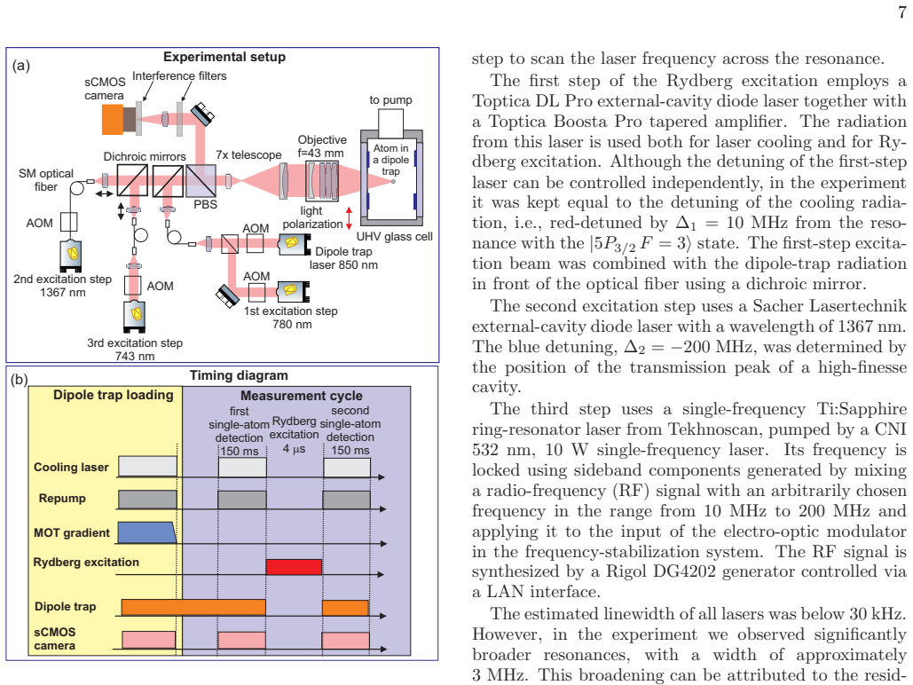
The central object is the five-level three-photon ladder (5S1/2, 5P3/2, 6S1/2, and the two Stark sublevels of 37P3/2), driven by 780, 1367, and 743 nm lasers, with the intermediate step coupled by a large Rabi frequency Ω23 ≫ Ω12, Ω34, Ω35. This ordering makes the three-photon resonance immune to light shifts, so Stark shifts and splittings can be read directly from the spectrum. Supporting machinery: the field from the eight segmented ring electrodes is computed by a Method-of-Moments solution of the electrostatic surface-charge integral equation, and the 37P3/2 Stark maps/polarizabilities come from a quasiclassical calculation (αP1/2 = 38.8 MHz/(V/cm)² and αP3/2 = 32.5 MHz/(V/cm)²), with a
Load-bearing premise
The chain converts measured frequency shifts into field strengths using theoretically computed polarizabilities of the 37P3/2 state (given as 38.8 and 32.5 MHz/(V/cm)^2, with 19.4 also used in one calibration) plus the claim that the three-photon resonance carries no light shift; if the polarizability values are inaccurate, or a residual light shift moves the resonances, all inferred field amplitudes and stray-field values shift together.
What would settle it
Measure the position of the 37P3/2 resonance while scanning the third-step laser intensity over a factor of about 10 at fixed voltage: if the resonance center moves by more than the linewidth (~3 MHz), the light-shift-free assumption fails. Alternatively, compare the inferred field Ex = 0.16U with an independent, non-Rydberg field sensor (e.g., microwave spectroscopy of a different transition) at the same location; a mismatch larger than the reported 15% would indicate incorrect polarizabilities.
If this is right
- Stray electric fields in glass vacuum cells can be measured and compensated in situ from the Rydberg excitation signal alone, without adding separate field sensors to the cell.
- Because the three-photon resonance is light-shift free, the field calibration is insensitive to laser intensity and polarization variations, removing a systematic error that complicates two-photon schemes.
- The same eight-electrode geometry and calibration method can generate a known DC field of arbitrary direction for Rydberg electrometry and for tuning long-range interactions between Rydberg atoms.
- The measured shifts validate the quasiclassically computed polarizabilities of the 37P3/2 state at fields below 2 V/cm, connecting the experiment to calculations of Rydberg radial matrix elements.
Where Pith is reading between the lines
- Extending to other alkali species and other nP states, this light-shift-free three-photon method should give a general way to map 3D fields inside compact UHV glass cells, where conventional field probes cannot fit.
- The roughly 15% discrepancy between measured and simulated field-per-volt (and larger for z) suggests the same Stark spectroscopy could also locate the atom's position within the electrode structure to sub-millimeter precision, not merely calibrate the field at one point.
- The paper does not report a direct intensity-dependence test of the light-shift-free assumption; varying the 743 nm laser power while holding voltage fixed would provide a clean, direct check.
- The observed ~3 MHz resonance broadening, blamed on residual magnetic fields, is the likely practical precision limit; improved magnetic compensation should sharpen the resonances and tighten the field calibration.
Editorial analysis
A structured set of objections, weighed in public.
Referee Report
Summary. The paper reports three-photon Stark spectroscopy of a single 87Rb atom trapped in an optical dipole trap inside an ultrahigh-vacuum octagonal glass cell with eight internal segmented ring electrodes. By applying voltages in configurations designed to produce electric fields along x, y, and z, the authors record shifts and splittings of the 37P3/2 Rydberg resonances, fit them with quadratic Stark dependencies to calibrate the field-per-volt coefficients, and estimate stray electric fields. The measured spectra are compared with a five-level Lindblad master-equation model using numerically calculated polarizabilities. The central claims are that the three-photon scheme avoids light shifts, that the eight-electrode geometry permits independent 3D field control and stray-field compensation, and that the measured spectra agree well with theory.
Significance. If correct, this work would provide a practical method for quantitative electric-field calibration and stray-field compensation in compact glass-cell Rydberg experiments, which is relevant for Rydberg-based quantum computing and electrometry. The use of a three-photon excitation scheme to avoid light shifts, the single-atom detection, and the availability of data on GitHub are positive features. The electrostatic Method-of-Moments simulation and the explicit five-level model are also concrete. However, the quantitative claims rest on an internally inconsistent polarizability value, and the absence of uncertainty estimates weakens the calibration statements. The comparison between experiment and theory is partially circular because the same theoretical polarizabilities are used both to calibrate the field and to generate the theory spectra.
major comments (4)
- [Sec. III vs Sec. V, Fig. 6(a)] There is a clear internal contradiction in the value of the polarizability used for the |mj|=1/2 component of 37P3/2. Section III states αP1/2 = 38.8 MHz/(V/cm)^2 from the numerically calculated Stark diagram, while Section V calibrates the x-direction data 'with αP1/2 = 19.4 MHz/(V/cm)^2'. Both labels refer to the same state. Because the Stark shift is −(1/2)αE^2, using 19.4 instead of 38.8 changes the inferred field by a factor of √2: the quoted calibration Ex = 0.16 U V/cm becomes 0.11 U V/cm, and the x stray field of 0.5 V/cm becomes 0.36 V/cm. These values feed directly into Fig. 7 and into the central claim of independent 3D control and stray-field compensation. The manuscript must resolve this inconsistency: identify which value is correct, explain the origin of the other value, and redo all x-direction calibrations and simulation inputs accordingly.
- [Sec. V, Fig. 6] The resonance-position data in Fig. 6 are shown without error bars, and no uncertainties are reported for the fitted quadratic coefficients, the derived calibration constants (Ex=0.16, Ey=0.16, Ez=0.185 V/cm per volt), or the inferred stray-field amplitudes. Since the paper makes precision claims ('high precision', '15% higher than calculations', agreement to within a stated percentage), quantitative uncertainties are essential. Please provide fit uncertainties, propagate them to the field calibrations and stray-field values, and state how the resonance centers were determined.
- [Sec. V, Figs. 7-9] The agreement between the measured and calculated spectra is partially circular: the voltage-to-field calibration is obtained by fitting measured Stark shifts using theoretically computed polarizabilities, and the same polarizabilities are then used to generate the 'theory' spectra. Thus agreement on absolute peak positions is enforced by construction. The paper should acknowledge this and provide an independent check if possible, e.g., a direct geometric calibration based only on the electrode simulation for at least one direction, or a measurement of a known transition frequency in zero field. This is especially important given the polarizability inconsistency noted above.
- [Sec. IV and Sec. V] The experimental resonances are reported to have a width of approximately 3 MHz, while the simulation includes only a 300 kHz pure dephasing rate at each transition. It is unclear how the theoretical curves in Figs. 7-9 reproduce the observed width. If additional broadening (e.g., laser linewidths, magnetic-field inhomogeneity, power broadening) is included in the plotted theory, this should be stated explicitly; otherwise the shape agreement needs justification. Please clarify the relationship between the observed 3 MHz width and the 300 kHz dephasing used in the model.
minor comments (5)
- [Sec. III, Eq. (15)] The text says the second laser (1367 nm) with Rabi frequency Ω12 drives the transition |1>→|2>, but in the Hamiltonian the second step should couple |2> and |3>; the symbol should presumably be Ω23.
- [Sec. I and Sec. V] Typographical errors: 'indvidually' (Sec. I) and 'spectrocopy' (Sec. V) should be corrected.
- [Sec. IV] The sign convention for 'blue detuning' ∆2 = −200 MHz is unusual; a blue detuning would normally be positive. Please clarify the sign convention used in Eq. (15).
- [Sec. V, Fig. 6 caption] The caption text 'voltage (V)' is repeated for the three panels without indicating the corresponding axis (x, y, z) inside the caption; add labels or a table for clarity.
- [Sec. V, z calibration] The z-direction calibration Ez = 0.185 V/cm per volt is about 33% higher than the electrostatic simulation (1.39 V/cm for 10 V, i.e., 0.139 V/cm per volt). The paper attributes this to imperfect axial positioning, but no quantitative estimate of the required displacement is given. A brief order-of-magnitude estimate would strengthen the discussion.
Circularity Check
Partial circularity: the theory spectra in Figs. 7–9 use electric fields calibrated from the same measured Stark shifts and polarizabilities, so agreement on absolute peak positions is enforced by construction; independent content remains in the splittings and in the electrostatic-simulation comparison.
specific steps
-
fitted input called prediction
[Sec. V (calibration) and Figs. 7–9; Sec. VII]
"From the quadratic approximation of the dependence in Fig. 6(a) with αP1/2 = 19.4 MHz/(V/cm)^2 we obtained the following calibration of the electric field related to applied voltage: Ex (V/cm) = 0.16 U (V). ... To confirm our findings, we numerically calculated the spectra of Rydberg excitation and compared them with the experiment. ... The positions and shapes of the experimentally recorded spectra are well described by our simple theoretical model."
The E-field values used as inputs to the theoretical spectra are obtained by inverting the very same measured Stark shifts with the same computed polarizabilities (Sec. V calibration and stray-field offsets from the fits in Fig. 6). Therefore the absolute resonance positions in the theory curves of Figs. 7–9 are constrained to match the fitted quadratic shifts; this part of the agreement is not an independent test. The non-trivial content is limited to the relative splittings, line shapes, and the voltage-to-field comparison with the independent electrostatic simulation (Sec. II).
full rationale
The calibration procedure itself—measuring Stark shifts and using theoretically computed polarizabilities to infer E—is a standard use of an external atomic-physics input, not circular. The paper also provides an independent benchmark: the measured calibration Ex ≈ 0.16 U V/cm is compared with the Method-of-Moments/Elmer electrostatic simulation (Sec. II predicts Ex = 1.43 V/cm at 10 V), and the moderate agreement supports the central claim of field control. The circularity is confined to the presentation of the calculated spectra in Figs. 7–9 as a confirmation: because the fields were calibrated from the same shifts, the absolute peak positions are anchored to the data by construction; the splittings and shapes remain genuine checks. The internal factor-of-two difference in the value labeled αP1/2 (38.8 MHz/(V/cm)^2 in Sec. III vs 19.4 MHz/(V/cm)^2 in Sec. V) appears to be a notation/definitional issue (Sec. III writes the Stark shift as −(1/2)αE^2) and is a correctness/consistency concern rather than a circularity. Self-citations to the authors' prior work on three-photon excitation and light shifts are contextual and are supplemented by the paper's own five-level Lindblad calculation, so they are not load-bearing here.
Axiom & Free-Parameter Ledger
free parameters (3)
- Stray electric field components used in simulations =
Ex = 0.5 V/cm, Ey = 0.05 V/cm, Ez = 0.12 V/cm
- Voltage-to-field calibration coefficients =
Ex = 0.16 U, Ey = 0.16 U, Ez = 0.185 U (V/cm per V)
- Dephasing rate from residual magnetic fields and laser linewidths =
300 kHz per transition
axioms (6)
- standard math Electrostatic field is governed by Laplace's equation with Dirichlet boundary conditions on the eight electrodes
- domain assumption The atom can be truncated to a five-level system with only two 37P3/2 Stark sublevels
- domain assumption The three-photon excitation scheme has negligible light shifts when Ω23 >> Ω12, Ω34, Ω35
- domain assumption Rydberg excitation is detected as loss from the optical dipole trap
- domain assumption The quasiclassical method [53] gives accurate polarizabilities for 37P3/2
- ad hoc to paper Stray electric fields in the simulation are determined from the same experimental data being compared
Cite this review
Pith. "Pith review of Three-dimensional three-photon Stark spectroscopy of a single Rb Rydberg atom in an ultrahigh-vacuum glass cell with eight electrodes." pith.science (2026). https://pith.science/paper/NIRYS36W
@misc{pith2026260715764,
  author       = {Pith},
  title        = {Pith review of: Three-dimensional three-photon Stark spectroscopy of a single Rb Rydberg atom in an ultrahigh-vacuum glass cell with eight electrodes},
  year         = {2026},
  howpublished = {\url{https://pith.science/paper/NIRYS36W}},
  note         = {Machine review of arXiv:2607.15764}
}
read the original abstract
Quantum computing and quantum simulation with ultracold neutral atoms require Rydberg excitation of individual atoms in atomic arrays. Rydberg states are extremely sensitive to external electric fields, therefore precise three-dimensional control of the electric field is essential. We performed a spectroscopic study of three-photon Rydberg excitation of a single Rb atom in an optical dipole trap in the presence of an external DC electric field. The field was generated by eight electrodes deposited on the inner surfaces of an ultrahigh-vacuum glass cell. The used three-photon scheme of laser excitation of Rydberg \textit{nP} states allows the Stark shift and the splitting of the resonances to be observed simultaneously, which simplifies calibration of the electric field. In addition, in the commonly used two-photon Rydberg excitation schemes, the light shifts can complicate accurate determination of the DC Stark shift, particularly when the external electric field is scanned across different spatial directions, and different Stark components are excited. These shifts are absent in the three-photon excitation scheme used in our experiment. We demonstrated the ability to independently tune the electric field along all three spatial directions and to compensate for stray electric fields. The measured three-photon spectra exhibit Stark shifts and splittings of the three-photon resonance that are in good agreement with theoretical calculations. These results are also of interest for Rydberg electrometry.
Figures




Reference graph
Works this paper leans on
-
[1]
N.-C. Chiu, E. C. Trapp, J. Guo, M. H. Abobeih, L. M. Stewart, S. Hollerith, P. Stroganov, M. Kalinowski, A. A. Geim, S. J. Evered, S. H. Li, L. M. Peters, D. Bluvstein, T. T. Wang, M. Greiner, V. Vuletic, and M. D. Lukin, Nature (2025)
2025
-
[2]
Analytic treatment of the singular self- and near-terms is essential for accu- racy [52]
may be used instead [51, 52]). Analytic treatment of the singular self- and near-terms is essential for accu- racy [52]. Once σ is known, the potential and field at any point r follow from superposition of the patch charges qi = σiAi: ϕ(r) = 1 4πε0 N∑ i=1 qi |r − ri| , (13) E(r) = −∇ϕ(r) = 1 4πε0 N∑ i=1 qi r − ri |r − ri|3 . (14) Other quantities follow di...
2000
-
[3]
into a Fredholm integral equation of the first kind for the un- known σ: 1 4πε0 ∫ S σ(r′) |r − r′| dS′ = Vk, r ∈ Sk, k = 1, . . . , Ne. (5) This is the electrostatic surface-charge integral equation; the single-layer potential is continuous across S, so no jump term appears (the jump appears only in the normal derivative, i.e. in the field). Equation (
-
[4]
Pichard, D
G. Pichard, D. Lim, E. Bloch, J. Vaneecloo, L. Bourachot, G.-J. Both, G. M´ eriaux, S. Du- tartre, R. Hostein, J. Paris, B. Ximenez, A. Sig- noles, A. Browaeys, T. Lahaye, and D. Dreon, Phys. Rev. Appl. 22, 024073 (2024)
2024
-
[5]
The MoM converts the integral equation Eq
is the starting point of the Method of Moments (MoM) [50, 51]. The MoM converts the integral equation Eq. ( 5) into a linear algebraic system by three steps [50, 51]: a. Basis-function expansion. The surface S is par- titioned into N small patches (boundary elements) {Si}N i=1, and the unknown density is expanded in a set of basis functions {fi}: σ(r′) ≈ ...
-
[6]
( 5) leaves a residual; we force its projection onto a set of testing functions {wj} to vanish, i.e
into Eq. ( 5) leaves a residual; we force its projection onto a set of testing functions {wj} to vanish, i.e. we take inner products ⟨wj , ·⟩ = ∫ S wj(r) (·) dS. Using point matching / collocation, wj(r) = δ(r − rj), the equation is enforced exactly at the patch centroids rj: N∑ i=1 Pji σi = V (rj ), j = 1, . . . , N, (8) with the potential-coefficient (mom...
-
[7]
6(a), but no splitting of the resonances is observed
When the electric field is directed along the x axis, which corresponds to the direction of laser polarization, the positions of the resonances are shifted, as shown in Fig. 6(a), but no splitting of the resonances is observed. When the electric field is directed along y or z axes, which are orthogonal to the direction of laser polarization, the resonances ...
-
[8]
This allowed us to calibrate the absolute position of zero Stark shift in Figs. 6-9. We estimated Rabi frequencies Ω 12/(2π) = 10 MHz and Ω 23/(2π) = 800 MHz from the laser power mea- surements and the laser beam waists. For the third step of laser excitation in the case of π polarization of the laser beam only the Stark component |4⟩ = |37P3/2 |mj| = 1 /...
-
[9]
Comparison between the theory and experimental records is shown in Fig. 7. In most cases our theoretical model correctly describes both the positions and shapes of the resonances. A more interesting case is when the electric field is scanned in orthogonal directions, allowing excitation of frequency (MHz) Single-atom retention 0,6 0,8 1,0 Account for 37P3/...
-
[10]
has a unique solution. 4 d. Off-diagonal terms ( j ̸= i). For well-separated patches the integrand is smooth and the centroid (monopole) approximation is used, Pji ≈ Ai 4πε0 |rj − ri| , A i = ∫ Si dS′, (11) i.e. patch i acts as a point charge qi = σiAi at its centroid. e. Diagonal terms ( j = i). Here rj ∈ Si and the kernel is singular (1 /|r − r′|), but t...
-
[11]
With the increase of the elec- tric field the resonances at first broaden due to the lifting of the degeneracy of two Stark components of Rydberg state, while the resonances remain overlapped. 10 frequency (MHz) Single-atom retention 0,4 0,6 0,8 1,0 Ez=1.18 V/cm 7V 0,4 0,6 0,8 1,0 Ez=1.0 V/cm6V 0,4 0,6 0,8 1,0 Account for 37P3/2 |mj=3/2| Account for 37P3/2 ...
-
[12]
H. J. Manetsch, G. Nomura, E. Bataille, K. H. Leung, X. Lv, and M. Endres, arXiv.2403.12021 10.48550/arXiv.2403.12021 (2024)
-
[13]
Gyger, M
F. Gyger, M. Ammenwerth, R. Tao, H. Timme, S. Snigirev, I. Bloch, and J. Zeiher, Phys. Rev. Res. 6, 033104 (2024)
2024
-
[14]
M. A. Norcia, H. Kim, W. B. Cairncross, M. Stone, A. Ryou, M. Jaffe, M. O. Brown, K. Barnes, P. Battaglino, T. C. Bohdanowicz, A. Brown, K. Cas- sella, C.-A. Chen, R. Coxe, D. Crow, J. Epstein, C. Griger, E. Halperin, F. Hummel, A. M. W. Jones, J. M. Kindem, J. King, K. Kotru, J. Lauigan, M. Li, M. Lu, E. Megidish, J. Marjanovic, M. Mc- Donald, T. Mittiga,...
2024
-
[15]
Jaksch, J
D. Jaksch, J. I. Cirac, P. Zoller, S. L. Rolston, R. Cˆ ot´ e, and M. D. Lukin, Phys. Rev. Lett 85, 2208 (2000)
2000
-
[16]
Gallagher, Rydberg atoms (Cambridge University Press, 1994)
T. Gallagher, Rydberg atoms (Cambridge University Press, 1994)
1994
-
[17]
Osterwalder and F
A. Osterwalder and F. Merkt, Phys. Rev. Lett. 82, 1831 (1999)
1999
-
[18]
Thiele, J
T. Thiele, J. Deiglmayr, M. Stammeier, J.-A. Ag- ner, H. Schmutz, F. Merkt, and A. Wallraff, Phys. Rev. A 92, 063425 (2015)
2015
-
[19]
Grimmel, M
J. Grimmel, M. Mack, F. Karlewski, F. Jessen, M. Reinschmidt, N. Sandor, and J. Fortagh, New Journal of Physics 17, 053005 (2015)
2015
-
[20]
Grimmel, M
J. Grimmel, M. Stecker, M. Kaiser, F. Karlewski, L. Torralbo-Campo, A. G¨ unther, and J. Fort´ agh, Phys. Rev. A 96, 013427 (2017)
2017
-
[21]
Kitson, W
P. Kitson, W. J. Chetcuti, G. Birkl, L. Amico, and J. Polo, Phys. Rev. Res. 8, 033010 (2026)
2026
-
[22]
Zhang, Y
H. Zhang, Y. Ma, K. Liao, W. Yang, Z. Liu, D. Ding, H. Yan, W. Li, and L. Zhang, Science Bulletin 69, 1515 (2024)
2024
-
[23]
D. H. Meyer, Z. A. Castillo, K. C. Cox, and P. D. Kunz, J. Phys. B: At. Mol. Opt. Phys 53, 034001 (2020)
2020
-
[24]
C. L. Degen, F. Reinhard, and P. Cappellaro, Rev. Mod. Phys. 89, 035002 (2017)
2017
-
[25]
I. I. Ryabtsev, D. B. Tretyakov, I. I. Beterov, and V. M. Entin, Phys. Rev. Lett. 104, 073003 (2010) . 12
2010
-
[26]
Nipper, J
J. Nipper, J. B. Balewski, A. T. Krupp, B. Butscher, R. L¨ ow, and T. Pfau, Phys. Rev. Lett. 108, 113001 (2012)
2012
-
[27]
D. B. Tretyakov, V. M. Entin, E. A. Yakshina, I. I. Beterov, C. Andreeva, and I. I. Ryabtsev, Phys. Rev. A 90, 041403 (2014)
2014
-
[28]
Y. Jiao, J. Bai, R. Song, S. Bao, J. Zhao, and S. Jia, Frontiers in Physics 27, 892542 (2022)
2022
-
[29]
Fredriksson and S
K. Fredriksson and S. Svanberg, Zeitschrift f¨ ur Physik A Atoms and Nuclei 281, 189 (1977)
1977
-
[30]
M. S. O’Sullivan and B. P. Stoicheff, Phys. Rev. A 31, 2718 (1985)
1985
-
[31]
T. W. Ducas, M. G. Littman, R. R. Freeman, and D. Kleppner, Phys. Rev. Lett. 35, 366 (1975)
1975
-
[32]
T. F. Gallagher, L. M. Humphrey, W. E. Cooke, R. M. Hill, and S. A. Edelstein, Phys. Rev. A 16, 1098 (1977)
1977
-
[33]
M. L. Zimmerman, M. G. Littman, M. M. Kash, and D. Kleppner, Phys. Rev. A 20, 2251 (1979)
1979
-
[34]
M. T. Frey, X. Ling, B. G. Lindsay, K. A. Smith, and F. B. Dunning, Rev. Sci. Instrum 64, 3649 (1993)
1993
-
[35]
I. M. Beterov and I. I. Ryabtsev, Journal of Experimental and Theoretical Physics Letters 68, 897 (1998)
1998
-
[36]
I. I. Ryabtsev and I. M. Beterov, Phys. Rev. A 61, 063414 (2000)
2000
-
[37]
Ryabtsev, D
I. Ryabtsev, D. Tretyakov, and I. Beterov, Journal of Physics B Atomic and Molecular Physics 36, 297 (2003)
2003
-
[38]
Hiller, S
M. Hiller, S. Yoshida, J. Burgd¨ orfer, S. Ye, X. Zhang, and F. B. Dunning, Phys. Rev. A 89, 023426 (2014)
2014
-
[39]
Zhang, F
X. Zhang, F. B. Dunning, S. Yoshida, and J. Burgd¨ orfer, Phys. Rev. A 92, 051402(R) (2015)
2015
-
[40]
Yoshida, J
S. Yoshida, J. Burgd¨ orfer, X. Zhang, and F. B. Dunning, Phys. Rev. A 95, 042705 (2017)
2017
-
[41]
Glick, J
J. Glick, J. R. Dickson, J. Wood, and P. Kunz, Phys. Rev. A 114, 012608 (2026)
2026
-
[42]
Grabowski, R
A. Grabowski, R. Heidemann, R. L¨ ow, J. Stuhler, and T. Pfau, Fortschritte der Physik 54, 765 (2006)
2006
-
[43]
T. Vogt, M. Viteau, A. Chotia, J. Zhao, D. Comparat, and P. Pillet, Phys. Rev. Lett. 99, 073002 (2007)
2007
-
[44]
Viteau, J
M. Viteau, J. Radogostowicz, M. G. Bason, N. Malossi, D. Ciampini, O. Morsch, and A. E., Optics Express 19, 6007 (2011)
2011
-
[45]
Ravets, H
S. Ravets, H. Labuhn, D. Barredo, L. Beguin, T. Lahaye, and A. Browaeys, Nat. Phys. 10, 914 (2014)
2014
-
[46]
Anand, C
S. Anand, C. E. Bradley, R. White, V. Ramesh, K. Singh, and H. Bernien, Nature Physics 20, 1744 (2024)
2024
-
[47]
Saßmannshausen, F
H. Saßmannshausen, F. Merkt, and J. Deiglmayr, Phys. Rev. A 87, 032519 (2013)
2013
-
[48]
J. Bai, S. Liu, J. Wang, J. He, and J. Wang, IEEE journal on selected topics in quantum electronics 26, 1600106 (2020)
2020
-
[49]
Cisternas, J
N. Cisternas, J. de Hond, G. Lochead, R. J. C. Spreeuw, H. B. v. L. van den Heuvell, and N. J. van Druten, Phys. Rev. A 96, 013425 (2017)
2017
-
[50]
Stecker, R
M. Stecker, R. Nold, L.-M. Steinert, J. Grim- mel, D. Petrosyan, J. Fort´ agh, and A. G¨ unther, Phys. Rev. Lett. 125, 103602 (2020)
2020
-
[51]
B. B. Zelener, S. A. Saakyan, V. A. Sautenkov, E. A. Manykin, B. V. Zelener, and V. E. Fortov, Journal of Experimental and Theoretical Physics 121, 950 (2015)
2015
-
[52]
Halter, A
C. Halter, A. Miethke, C. Sil- lus, A. Hegde, and A. G¨ orlitz, Journal of Physics B: Atomic, Molecular and Optical Physics 56, 055001 (2023)
2023
-
[53]
Electric field control for experiments with atoms in Rydberg states
A. Panja, Y. Wang, X. Wang, J. Wang, S. Sub- hankar, and Q.-Y. Liang, arXiv:2409.11865 10.48550/arXiv.2409.11865 (2024)
work page internal anchor Pith review Pith/arXiv arXiv doi:10.48550/arxiv.2409.11865 2024
-
[54]
T. A. Johnson, E. Urban, T. Henage, L. Isen- hower, D. D. Yavuz, T. G. Walker, and M. Saffman, Phys. Rev. Lett. 100, 113003 (2008)
2008
-
[55]
Saffman, T
M. Saffman, T. G. Walker, and K. Mølmer, Rev. Mod. Phys. 82, 2313 (2010)
2010
-
[56]
N. N. Bezuglov, I. I. Beterov, A. Cinins, K. Miculis, V. M. Entin, P. I. Betleni, G. Suliman, V. V. Gromyko, D. B. Tretyakov, E. A. Yakshina, and I. I. Ryabtsev, Phys. Rev. A 112, 063103 (2025)
2025
-
[57]
R. Ding, J. D. Whalen, S. K. Kanungo, T. C. Kil- lian, F. B. Dunning, S. Yoshida, and J. Burgd¨ orfer, Phys. Rev. A 98, 042505 (2018)
2018
-
[58]
C. S. Hofmann, G. G¨ unter, H. Schempp, N. L. M. M¨ uller, A. Faber, H. Busche, M. Robert-de Saint-Vincent, S. Whitlock, and M. Weidem¨ uller, Frontiers of Physics 121, 571 (2014)
2014
-
[59]
R. F. Harrington, Field Computation by Moment Meth- ods (IEEE Press, 1993) pp. 1–219
1993
-
[60]
W. C. Gibson, The Method of Moments in Electromag- netics (Taylor and Francis Group, LLC, 2008) pp. 1–272
2008
-
[61]
S. M. Rao, T. K. Sarkar, and R. F. Harrington, IEEE Transactions on Microwave Theory and Techniques 32, 1441 (1984)
1984
-
[62]
Kaulakys, J
B. Kaulakys, J. Phys. B: At. Mol. Opt. Phys. 28, 4963 (1995)
1995
-
[63]
ˇSibali´ c, J
N. ˇSibali´ c, J. D. Pritchard, C. S. Adams, and K. J. Weatherill, Computer Physics Communications 220, 319 (2017)
2017
-
[64]
I. I. Beterov, I. I. Ryabtsev, D. B. Tretyakov, and V. M. Entin, Phys. Rev. A 79, 052504 (2009)
2009
-
[65]
Beterov, E
I. Beterov, E. Yakshina, G. Suliman, P. Betleni, A. Prilutskaya, D. Skvortsova, T. Zagirov, D. Tretyakov, V. Entin, N. Bezuglov, and I. Ryabtsev, Journal of Experimental and Theoretical Physics 166, 516 (2024)
2024
-
[66]
I. I. Sobelman, Atomic Spectra and Radiative Transitions , 2nd ed., Springer Series on Atoms+Plasmas, Vol. 12 (Springer-Verlag, Berlin Heidelberg, 1992) chapter 9 details the explicit calculations for relative amplitudes of fine-structure components
1992
-
[67]
I. I. Beterov, E. A. Yakshina, D. B. Tretyakov, N. V. Al’yanova, D. A. Skvortsova, G. Suli- man, , T. Zagirov, , V. Entin, and I. Ryabtsev, Journal of Experimental and Theoretical Physics 137, 246 (2023)
2023
-
[68]
Hattermann, M
H. Hattermann, M. Mack, F. Karlewski, F. Jessen, D. Cano, and J. Fort´ agh, Phys. Rev. A 86, 022511 (2012)
2012
-
[69]
J. A. Sedlacek, E. Kim, S. T. Rittenhouse, P. F. Weck, H. R. Sadeghpour, and J. P. Shaffer, Phys. Rev. Lett. 116, 133201 (2016)
2016
-
[70]
R. P. Abel, C. Carr, U. Krohn, and C. S. Adams, Phys. Rev. A 84, 023408 (2011)
2011
-
[71]
Davtyan, S
D. Davtyan, S. Machluf, M. L. Soudijn, J. B. Naber, N. J. van Druten, H. B. van Linden van den Heuvell, and R. J. C. Spreeuw, Phys. Rev. A 97, 023418 (2018)
2018
-
[72]
K. S. Chan, M. Siercke, C. Hufnagel, and R. Dumke, Phys. Rev. Lett. 112, 026101 (2014)
2014
-
[73]
Mamat, C
B. Mamat, C. Sheng, Y.-Q. Zhang, J.-Y. Hou, P. Xu, K.-P. Wang, J. Zhuang, M.-R. Wei, M. Liu, J. Wang, X.-D. He, and M.-S. Zhan, Phys. Rev. Appl. 22, 064021 (2024)
2024
-
[74]
Efficient photo-ionizing elimination of detrimental electric fields for Rydberg atoms
Z.-C. Deng, H.-N. Lin, Y.-C. Duan, Q. Zhang, X.-C. Cheng, Y. Liu, Z.-Y. Yuan, J. Li, P. Liu, Z. Wu, C.-Y. Lu, J. Rui, and J.-W. Pan, https://arxiv.org/abs/2607.08418 10.48550/arXiv.2607.08418 (2026)
work page internal anchor Pith review Pith/arXiv arXiv doi:10.48550/arxiv.2607.08418 2026
-
[75]
J. Miles, M. T. Lichtman, A. M. Scott, J. Scott, S. A. Norrell, M. J. Bedalov, D. A. Belknap, D. C. Cole, 13 S. Y. Eubanks, M. Gillette, P. Gokhale, J. Goldwin, G. T. Hickman, M. Iliev, R. A. Jones, K. W. Kuper, D. Mason, P. T. Mitchell, J. D. Murphree, N. A. Neff- Mallon, T. W. Noel, A. G. Radnaev, I. V. Vinogradov, and M. Saffman, https://arxiv.org/abs/26...
arXiv 2026
-
[76]
V. M. Entin, E. A. Yakshina, , D. B. Tretyakov, I. I. Beterov, and I. I. Ryabtsev, J. Exp. Theor. Phys. 116, 721 (2013)
2013
-
[77]
I. I. Ryabtsev, I. I. Beterov, D. B. Tretyakov, V. M. Entin, and E. A. Yakshina, Phys. Usp. 59, 196 (2016)
2016
-
[78]
E. A. Yakshina, D. B. Tretyakov, V. M. Entin, I. I. Beterov, and I. I. Ryabtsev, Quantum Electronics 48, 886 (2018)
2018
-
[79]
D. B. Tretyakov, E. A. Yakshina, V. M. Entin, I. I. Beterov, and I. I. Ryabtsev, Quantum Electronics 52, 513 (2022)
2022
-
[80]
J. Bai, Y. Jiao, Y. He, R. Song, J. Zhao, and S. Jia, Optics Express 30, 16748 (2022)
2022
This paper was first reviewed by deepseek-v4-flash on August 1, 2026.
discussion (0)
Sign in with ORCID, Apple, or X to comment. Anyone can read and Pith papers without signing in.