REVIEW 3 major objections 5 minor 1 cited by
Cosmological stasis would leave a measurable imprint in the gravitational-wave background.
Reviewed by Pith at T0; open to challenge. T0 means a machine referee read the full paper against a public rubric. the ladder, T0–T4 →
T0 review · deepseek-v4-flash
2026-08-01 15:22 UTC pith:JVJSTQUA
load-bearing objection Useful forecast with a genuinely nice g* fine-structure analysis, but the abstract's 'entire parameter space' detection claim for ws > 1/3 is stronger than the PLS criterion actually supports. the 3 major comments →
Detecting Cosmological Stasis with Future Gravitational Wave Observatories
The pith
A machine-rendered reading of the paper's core claim, the machinery that carries it, and where it could break.
Core claim
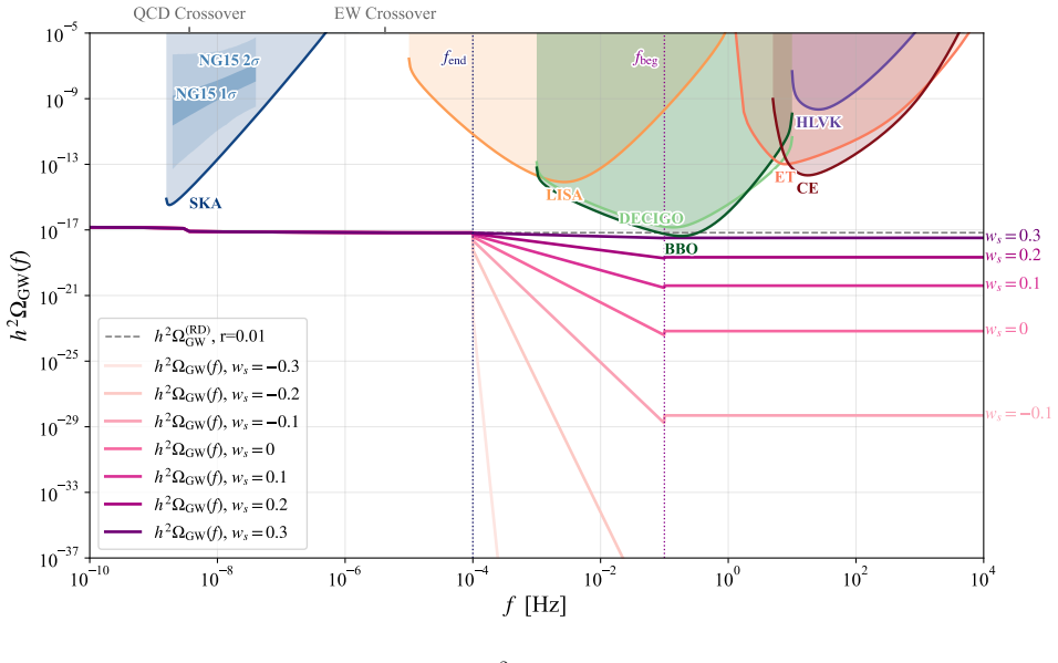
The paper's central claim: a cosmological stasis epoch imprints a calculable three-piece distortion on the inflationary gravitational wave background — a flat plateau below f_end, a power-law band with tilt α(w_s) = 2(3w_s − 1)/(1 + 3w_s), and a tilted plateau above f_beg, with the amplitude step at f_end set by the Bessel coefficient C^2(ν(w_s)). That coefficient is tied to α by a universal relation C^2 = C^2(α), so α and C^2 are independently measurable and the spectrum is falsifiable without knowing w_s in advance. Over detector sensitivity curves, the template gives the shortest detectable stasis duration ΔN_min(w_s, r). Result: BBO detects enhanced stasis across the whole parameter spac
What carries the argument
The closed-form piecewise spectral template of Eq. (4), derived in the companion work, built on the exact Bessel solution of the tensor mode equation during constant-w_s expansion. Its load-bearing pieces: the Bessel amplitude coefficient C^2(ν), the spectral tilt α(w_s) = 2(3w_s − 1)/(1 + 3w_s), and the two break frequencies f_end and f_beg = f_end exp[(1 + 3w_s)ΔN/2]. The universal consistency relation C^2 = C^2(α) (Eq. 7) is what makes the signature specific to stasis: the slope and the step height must land on one curve. The paper places this template against power-law integrated sensitivity curves to derive ΔN_min(w_s, r) detectability maps.
Load-bearing premise
The detectability claims inherit the companion paper's template as exact — the Bessel amplitude C^2(ν), the tilt α(w_s), and the sharp breaks at f_end and f_beg are assumed without re-derivation here; if that template's normalization or matching is off, the ΔN_min maps and detector reach shift.
What would settle it
A future BBO/DECIGO measurement of the IGWB in the 0.01–1 Hz band that shows no break or shoulder at the predicted f_end, no power-law segment with the predicted slope α(w_s), or whose measured slope-step pair (α, C^2) lies off the universal curve C^2 = C^2(α) would falsify the paper's central claim. Concretely, for canonical stasis near w_s ≈ 0 (matter-like), the template predicts a roughly 44% downward step at f_end; its absence for a long stasis epoch in that band would rule out canonical stasis in that parameter region.
If this is right
- BBO and DECIGO, not LISA or ET, become the main instruments for stasis in the IGWB; BBO covers suppressed stasis for w_s ≈ 0.2 at r = 0.036 and enhanced stasis over the full (w_s, ΔN) plane at r = 0.01.
- Enhanced stasis decouples from the tensor amplitude: near the kination limit the BBO threshold drops to r ≈ 10^-9, far below projected CMB reach.
- Standard Model phase transitions impose fixed spectral steps (about 20% at ~2.6 × 10^-6 Hz, about 53% at ~3.6 × 10^-9 Hz) that must be modeled inside the stasis band and can serve as calibration.
- A finite-width end-of-stasis transition rounds the f_end break over Δ ln f = 3(1 + w_s)/4 × ΔN_trans without destroying the consistency relation as long as ΔN_stasis ≫ ΔN_trans.
- A measured slope alone only hints at stasis; measuring both α and C^2 lets one test the universal curve and reject mimics.
Where Pith is reading between the lines
- The ΔN_min maps imply a concrete search strategy: concentrate on the 0.01–1 Hz band, since that is where the detection threshold is lowest, and treat a null result as a bound on (w_s, ΔN, T_end, r) combinations rather than just a limit on r.
- The fixed g* steps could be exploited as in-situ calibrators; a mismatch between observed and predicted step amplitude would flag either new relativistic degrees of freedom at the corresponding temperature or detector systematics.
- If the Bogoliubov oscillations predicted for sharp transitions (ΔN_trans ≈ 1) are computed, the shoulder width could discriminate between decaying-tower, PBH, and dynamical-scalar realizations of stasis.
- The near-kination r_min ≈ 10^-9 result means a BBO detection would probe physics well beyond the reach of CMB-S4 and LiteBIRD; conversely, absence of the feature would push any enhanced-stasis realization to small w_s or short durations.
Editorial analysis
A structured set of objections, weighed in public.
Referee Report
Summary. This paper maps the inflationary gravitational wave background (IGWB) distortion predicted during cosmological stasis onto the projected sensitivity bands of current and future gravitational-wave observatories. Using a closed-form piecewise template from a companion paper, it computes the spectrum for four stasis scenarios across three representative frequency bands, includes the Standard Model g_* fine structure as fixed calibration features, and models the finite-width end-of-stasis transition phenomenologically. The headline claims are that for suppressed spectra (w_s < 1/3) BBO can detect the stasis feature for w_s ≳ 0.2 at r = 0.036, and for enhanced spectra (w_s > 1/3) BBO can detect it across the entire (w_s, ΔN) parameter space at r = O(0.01), with r as low as 10^{-9} near kination. Detectability is assessed with power-law integrated sensitivity (PLS) curves using a criterion that both the tilted stasis band and at least one adjacent plateau cross the PLS curve.
Significance. If the detectability claims hold, the paper identifies BBO and DECIGO as decisive instruments for testing cosmological stasis and provides a concrete observational program: three independent observables (spectral tilt, amplitude step, and transition smoothing width) plus fixed SM g_* steps as calibration features. The paper is a forward-modeling forecast, not a fit, so there is no circularity in applying the companion template. Strengths include the parameter-free smoothing formula of Eq. (21), the explicit treatment of g_* fine structure, and the open acknowledgment of PLS limitations. The main weakness is that the central 'entire parameter space' claim for enhanced spectra rests on a detectability criterion that may certify only that the overall background is above noise, not that the stasis break/tilt is resolvable.
major comments (3)
- [Sec. IVB, Eq. (13), Fig. 4, and abstract] The PLS-crossing criterion produces ΔN_min → 0 for w_s > 1/3 at r = O(0.01) whenever the RD baseline itself exceeds the PLS floor. For r = 0.01, h²Ω_GW^(RD) ≈ 6.8×10⁻¹⁸, above BBO's PLS minimum ≈ 4×10⁻¹⁸; the stasis band is C²·baseline ≥ baseline and the pre-stasis plateau is further enhanced, so both required pieces cross the PLS curve for arbitrarily small ΔN. A PLS crossing at SNR ≈ 1 certifies only that each segment is individually detectable as an isolated power law, not that the fractional break between them is resolvable: a step of relative height δ is measured with SNR ≈ δ/√2, so even the maximal canonical step (δ ≈ 44%) is marginal. The maps therefore trace where the overall background is above noise rather than where the stasis feature is detectable. This is acknowledged in the Sec. IVB Note, but the abstract and Sec. IVC2 state the stronger claim. Please add a model-comparison
- [Sec. IVC2 and Figs. 8–10] The statement that 'BBO can detect the stasis feature across the entire w_s ∈ (1/3,1) parameter space at r=0.01' is internally qualified by the paper's own observation that in Band III only the enhancement is measurable, not the amplitude step C², so the consistency relation C²=C²(α) cannot be tested. A feature that is just an elevated power-law excess is not stasis-specific. The detectability maps should distinguish between 'spectral excess above noise' and 'stasis feature verified through the consistency relation'. This distinction exists in the narrative but is absent from the abstract and Fig. 4.
- [Eq. (4) and all subsequent forecasts] Every numerical result inherits the companion-paper template [1] — C²(ν), α(w_s), and sharp piecewise matching at f_end and f_beg — without independent re-derivation or validation in this manuscript. The companion paper reportedly cross-checks against [3], but that check is not reproduced here. If any normalization or matching error exists in [1], all ΔN_min boundaries shift. This is load-bearing; state explicitly that all quantitative results are conditional on [1] and include a short reproducibility check.
minor comments (5)
- [Sec. IIB, Eq. (6)] The notation g_*0 ≡ g_*(T_beg) is confusing, since g_*0 conventionally denotes the present-day value. Use a subscript such as g_*^beg or define more carefully.
- [Fig. 12 caption vs. text] The text says f_end = 10⁻¹ Hz, while the caption says f_end = 2×10⁻¹ Hz. Please make these consistent.
- [Table I] The header 'Eraw s' appears garbled; it should be 'w_s'.
- [Sec. IVB Note] The third caveat says the maps show the envelope over instruments. This makes it difficult to infer BBO's specific reach from Fig. 4 alone; consider marking which instrument is most sensitive at each point in a separate panel.
- [Appendix A and Figs. 13–15] The vertical axis in the vacuum-energy/matter plots extends to 10⁻⁶², vastly below detector sensitivities; consider limiting the plotted range so that the shape of the feature in the observable band is visible.
Circularity Check
Forecasts are forward-modeling applications of the companion-paper template, not fits; the main circularity risk is the PLS-based detectability criterion, which the authors themselves flag as approximate for broken power laws, plus the load-bearing self-citation of [1].
specific steps
-
other
[Sec. IVB (Detectability maps), around Eq. (13) and the Note following it; abstract claims of full-parameter-space detectability]
"Requiring only that the tilted stasis band [fend, fbeg] rise above the PLS curve is sufficient to measure the slope α and hence ws, but as emphasized in Sec. IVA a measured slope alone is a hint rather than a test: the consistency relation C2 = C2(α) of eq. (7) is what makes the signature specific to stasis, and it requires the amplitude step at fend to be measurable independently. ... First, PLS curves are constructed for pure power-law backgrounds [18], so a broken power law that crosses one attains SNR∼ρthr only approximately; the maps are accurate at the level of the shape of the detectabl"
The central 'entire parameter space at r=O(0.01)' enhancement claim is generated by a crossing criterion that is acknowledged to be only an SNR proxy for resolvability of a broken power law. When the RD baseline itself already lies above the PLS minimum (as it does for BBO at r=0.01), any positive stasis tilt or plateau yields PLS crossing for arbitrarily small ΔN, so ΔNmin→0 in Fig. 4 maps where the overall background is above noise rather than where the stasis feature (break + tilt) is separately resolvable. The paper itself defers a Fisher/model-comparison analysis, so the literal 'entire parameter space' wording outruns the quoted caveat.
-
self citation load bearing
[Sec. II (Summary of the stasis GW template), Eqs. (1)-(7); Sec. IVA/IVC; Sec. VI; abstract]
"Using the closed-form piecewise spectral template derived in the companion paper [1], we generate detectability maps for four stasis scenarios... In the companion paper [1] we derived this closed-form template, established the consistency relation C2 = C2(α)... and validated the framework against the numerical PBH-stasis calculation of [3]."
All detectability maps, ΔNmin values, and r-min claims inherit the companion paper's template (normalization C2(ν), tilt α(ws), and sharp piecewise breaks) without re-derivation in this paper. However, the template is independently supported: [1] validates it against the numerical PBH-stasis calculation of [3], which is a distinct group, and the present paper does not fit the template to data. So the self-citation is load-bearing but not circular: it transfers a previously derived and externally validated input. This is the heaviest self-citation in the paper and the one a referee would want to see reproduced, but on the evidence given it is not a definitional reduction.
full rationale
The paper is a forward-modeling forecast, not a fit, and I find no step in which a predicted quantity is constructed from the same data it is said to predict. The stasis template (Eq. 4) is taken from the authors' companion paper [1], but [1] is said to validate it against the independent numerical PBH-stasis calculation of [3], so the template is not merely an ansatz imported through self-citation. The g* fine structure (Sec. III) is a parameter-free application of SM thermodynamics tables, and the transition smoothing (Sec. V) is a kinematic integral w(N) over a single width parameter — neither reduces to the claimed outputs. The genuinely questionable step is the detectability criterion in Sec. IVB: the ΔNmin maps and the headline 'entire (ws,ΔN) parameter space' claims are produced by asking whether the flat stasis band and an adjacent plateau cross the PLS curve, which is explicitly a broken-power-law misuse of a pure-power-law sensitivity curve. Because the RD baseline at r=0.01 already lies above BBO's PLS minimum, the enhancement maps largely trace overall amplitude rather than resolvability of the stasis break and tilt, so the 'entire parameter space' claim is not yet supported by the paper's own criterion. That is a correctness/calibration concern about the detection statistic, however, not a circularity of the type 'prediction equals input by construction': the maps are derived from the template and detector curves, not fitted back to them, and the paper itself states that a Fisher analysis is needed. On the circularity scale, the self-citation of [1] is load-bearing but externally anchored, and the PLS caveat is explicit; I therefore score 3 rather than higher. A central derivation that is independently parameter-free would be a 0-2; here the over-broad abstract wording based on an admittedly approximate criterion and the heavy dependence on the same-authors template justify a modest score, but no definitional or fitted-input circularity is established.
Axiom & Free-Parameter Ledger
free parameters (6)
- r (tensor-to-scalar ratio) =
0.01 baseline; 0.036 Planck upper limit; down to 1e-9 in Fig. 11
- f_end (lower break frequency anchor) =
1e-4, 1e-9, 1e-2 Hz (the three bands of Table II)
- ΔN_stasis (stasis duration) =
scanned; ΔN_min derived by threshold inversion of Eq. (13)
- ws (stasis equation of state) =
scanned over (-1/3, 1)
- ΔN_trans (transition width) =
assumed O(1); plotted at 0, 1, 3, 6 in Fig. 12
- SNR threshold ρ_thr = 1 and T_obs = 4 yr =
standard PLS configurations from Schmitz [18]
axioms (5)
- domain assumption Closed-form piecewise stasis template (Eq. 4) from companion paper [1]: Bessel coefficient C^2(ν), tilt α(ws), piecewise form
- domain assumption Nearly scale-invariant primordial tensor spectrum with pivot k* = 0.05 Mpc^-1
- domain assumption SM g*(T) thermal history of Laine-Meyer [17], with sharp QCD crossover and smooth EW roll-off
- domain assumption PLS curves of Schmitz [18] with ρ_thr = 1, T_obs = 4 yr are a valid proxy for detectability of a broken power law
- ad hoc to paper Symmetric monotonic w(N) profiles interpolating ws to 1/3 give the closed-form smoothing width Eq. (21)
read the original abstract
We map the observational predictions of cosmological stasis in the inflationary gravitational wave background onto the sensitivity bands of current and planned gravitational wave detectors. Using the closed-form piecewise spectral template derived in the companion paper, we generate detectability maps for four stasis scenarios: canonical, dynamical scalar, vacuum-energy/matter, and vacuum-energy/radiation across the frequency bands probed by NANOGrav, SKA, LISA, DECIGO, BBO, the Einstein Telescope, and Cosmic Explorer. For scenarios in which the spectrum is suppressed, $w_s < 1/3$, the stasis feature is detectable by BBO in the region of $(w_s,\Delta N)$ parameter space in which $w_s\gtrsim 0.2$ for tensor-to-scalar ratios close to the Planck upper limit, r = 0.036. For scenarios in which the spectrum is enhanced, $w_s > 1/3$, the stasis feature is detectable by BBO across the entire $(w_s,\Delta N)$ parameter space for tensor-to-scalar ratios of $O(0.01)$. We characterize the Standard Model (SM) $g_*$ fine structure of the IGWB, showing that SM phase transitions introduce spectral steps of $\approx 20\%$ (electroweak, at $\sim 2.6\times10^{-6}$~Hz) and $\approx 53\%$ (QCD, at $\sim 3.6\times 10^{-9}$~Hz). For stasis scenarios with end-of-stasis temperatures below the QCD scale these steps fall inside the stasis band and constitute additional spectral features that complement the primary signature. Finally, we model the finite-width end-of-stasis transition phenomenologically, demonstrating that the spectral break at $f_{end}$ is smoothed over a log-frequency window $\Delta N_\mathrm{trans}\times 3(1+w_s)/4$, and that the consistency relation $C^2=C^2(\alpha)$ remains testable provided $\Delta N_\mathrm{stasis}\gg \Delta N_\mathrm{trans}$, a condition easily satisfied for all scenarios of phenomenological interest.
Figures




Forward citations
Cited by 1 Pith paper
-
The Pull of Stasis: A Study of the Dynamics of the Thermal Stasis Attractor
An explicit three-scalar model realizes a thermal stasis attractor with a finite lifetime, whose fast and slow trajectories make the duration of stasis strongly initial-condition dependent.
Reference graph
Works this paper leans on
-
[1]
Canonical stasis(0≤w s <1/3)17
-
[2]
fine structure
Dynamical scalar stasis(1/3< ws <1)18 D. Consistency with the∆Neff bound 20 E. Which microphysical realizations land where? 23 V. End-of-stasis transition: a phenomenological treatment 25 A. The transition width∆Ntrans 26 B. How the transition smooths the spectrum 26 Deep sub-horizon modes are unaffected 27 Sharp transitions and Bogoliubov oscillations 28...
-
[3]
The Bessel amplitude satisfiesC 2 ∈(9/16,1), so the spectrum steps down by at most ∼44%atf end
Canonical stasis(0≤w s <1/3) Canonical stasis [2] spansw s ∈[0,1/3), givingα∈(−2,0): the stasis band is suppressed relative to the RD baseline (a notch), with suppression deepening asws →0(matter domina- tion). The Bessel amplitude satisfiesC 2 ∈(9/16,1), so the spectrum steps down by at most ∼44%atf end. The pre-stasis plateau is additionally suppressed ...
-
[4]
Unit of Excellence Maria de Maeztu 2020-2023
Dynamical scalar stasis(1/3< w s <1) Dynamical scalar stasis [5] arises when a scalar field sustains a fixed equation of statews ∈ (1/3,1)through a potential-dominated attractor. The key distinction from the canonical and vacuum-energy scenarios is the sign of the spectral tilt:α(ws)>0forw s >1/3, so the stasis band isenhancedrelative to the radiation-dom...
2020
-
[5]
G. Barenboim and A.-K. Burns, Gravitational Wave Signatures of Cosmological Stasis: A Unified Spectral Template (2026), arXiv:2607.03537 [hep-ph]
Pith/arXiv arXiv 2026
-
[6]
K. R. Dienes, L. Heurtier, F. Huang, D. Kim, T. M. Tait, and B. Thomas, Phys. Rev. D105, 023530 (2022), arXiv:2111.04753 [astro-ph.CO]
Pith/arXiv arXiv 2022
-
[7]
K. R. Dienes, L. Heurtier, F. Huang, D. Kim, T. M. Tait, and B. Thomas, Phys. Rev. D112, 083546 (2025), arXiv:2212.01369 [astro-ph.CO]
arXiv 2025
-
[8]
K. R. Dienes, L. Heurtier, F. Huang, T. M. Tait, and B. Thomas, Phys. Rev. D112, 083547 (2025), arXiv:2510.06551 [astro-ph.CO]
arXiv 2025
-
[9]
K. R. Dienes, L. Heurtier, F. Huang, T. M. Tait, and B. Thomas, Phys. Rev. D110, 123514 (2024), arXiv:2406.06830 [astro-ph.CO]
Pith/arXiv arXiv 2024
-
[10]
J. Barber, K. R. Dienes, and B. Thomas, Phys. Rev. D110, 123515 (2024), arXiv:2408.16255 [astro-ph.CO]. 31
Pith/arXiv arXiv 2024
-
[11]
J. Barber, K. R. Dienes, and B. Thomas, Phys. Rev. D111, 063519 (2025), arXiv:2412.09123 [astro-ph.CO]
Pith/arXiv arXiv 2025
- [12]
-
[13]
A. J. Long, B. Shams Es Haghi, and M. Venegas, JCAP01, 037, arXiv:2506.04502 [hep-ph]
-
[14]
J. Halverson and S. Pandya, Phys. Rev. D110, 075041 (2024), arXiv:2408.00835 [hep-ph]
Pith/arXiv arXiv 2024
-
[15]
A. A. Starobinsky, JETP Lett.30, 682 (1979)
1979
-
[16]
V. A. Rubakov, M. V. Sazhin, and A. V. Veryaskin, Phys. Lett. B115, 189 (1982)
1982
-
[17]
L. A. Boyle and P. J. Steinhardt, Phys. Rev. D77, 063504 (2008), arXiv:astro-ph/0512014 [astro- ph]
Pith/arXiv arXiv 2008
-
[18]
Planck Collaboration, Y. Akrami, F. Arroja, M. Ashdown, J. Aumont,et al., Astron. Astrophys. 641, A10 (2020), arXiv:1807.06211 [astro-ph.CO]
Pith/arXiv arXiv 2020
-
[19]
BICEP/Keck Collaboration, Phys. Rev. Lett.127, 151301 (2021), arXiv:2110.00483 [astro- ph.CO]
arXiv 2021
-
[20]
Y. Watanabe and E. Komatsu, Phys. Rev. D73, 123515 (2006), arXiv:astro-ph/0604176
Pith/arXiv arXiv 2006
- [21]
-
[22]
K. Schmitz, JHEP01, 097, compilation of power-law-integrated sensitivity curves for current and proposed GW detectors; data archived at Zenodo:3689582, arXiv:2002.04615 [hep-ph]
Pith/arXiv arXiv 2002
-
[23]
Arzoumanianet al.(NANOGrav), Astrophys
Z. Arzoumanianet al.(NANOGrav), Astrophys. J. Lett.905, L34 (2020), arXiv:2009.04496 [astro- ph.HE]
Pith/arXiv arXiv 2020
-
[24]
S. Chenet al.(EPTA), Mon. Not. Roy. Astron. Soc.508, 4970 (2021), arXiv:2110.13184 [astro- ph.HE]
Pith/arXiv arXiv 2021
-
[25]
G. Janssen, G. Hobbs, M. McLaughlin, C. Bassa, A. Deller, M. Kramer, K. Lee, C. Mingarelli, P. Rosado, S. Sanidas, A. Sesana, L. Shao, I. Stairs, B. Stappers, and J. P. W. Verbiest, PoS AASKA14, 037 (2015), arXiv:1501.00127 [astro-ph.IM]
Pith/arXiv arXiv 2015
-
[26]
Amaro-Seoaneet al.(LISA), Laser Interferometer Space Antenna (2017), arXiv:1702.00786 [astro-ph.IM]
P. Amaro-Seoaneet al.(LISA), Laser Interferometer Space Antenna (2017), arXiv:1702.00786 [astro-ph.IM]
Pith/arXiv arXiv 2017
-
[27]
Kawamuraet al., Class
S. Kawamuraet al., Class. Quant. Grav.28, 094011 (2011)
2011
-
[28]
V. Corbin and N. J. Cornish, Class. Quant. Grav.23, 2435 (2006), arXiv:gr-qc/0512039
Pith/arXiv arXiv 2006
-
[29]
Punturoet al., Classical and Quantum Gravity27, 194002 (2010)
M. Punturoet al., Classical and Quantum Gravity27, 194002 (2010)
2010
-
[30]
D. Reitzeet al., Bull. Am. Astron. Soc.51, 035 (2019), arXiv:1907.04833 [astro-ph.IM]
Pith/arXiv arXiv 2019
-
[31]
G.Agazieet al.(NANOGrav),Astrophys.J.Lett.951,L8(2023),arXiv:2306.16213[astro-ph.HE]. 32
Pith/arXiv arXiv 2023
-
[32]
K. N. Abazajianet al.(CMB-S4),CMB-S4 Science Book, First Edition(2016) arXiv:1610.02743 [astro-ph.CO]
Pith/arXiv arXiv 2016
- [33]
-
[34]
C. Caprini and D. G. Figueroa, Class. Quant. Grav.35, 163001 (2018), arXiv:1801.04268 [astro- ph.CO]
Pith/arXiv arXiv 2018
-
[35]
K. R. Dienes, L. Heurtier, F. Huang, T. M. Tait, and B. Thomas, Phys. Rev. D109, 083508 (2024), arXiv:2309.10345 [astro-ph.CO]. Appendix A: V acuum-energy/matter stasis (−1/3< w s <0) In the vacuum-energy/matter scenario of [31] (Sec. III therein), the stasis attractor sustains a non-zero vacuum-energy fraction alongside matter, giving an effective equati...
Pith/arXiv arXiv 2024
discussion (0)
Sign in with ORCID, Apple, or X to comment. Anyone can read and Pith papers without signing in.