REVIEW 4 major objections 5 minor 37 references
Deterministic classifier-free guidance does not sample the product distribution p^ω q^{1−ω}; its true distribution is the target density times an exponential path-integral correction that accumulates score discrepancies along the sampling t
Reviewed by Pith at T0; open to challenge. T0 means a machine referee read the full paper against a public rubric. the ladder, T0–T4 →
T0 review · deepseek-v4-flash
2026-08-01 11:53 UTC pith:XBVBVWMQ
load-bearing objection The path-integral characterization of CFG's sampling distribution is real and the toy verification is convincing; the DG-CFG schedule, however, is a heuristic built on an untested neglect of the geometry term. the 4 major comments →
Analytic Distribution of Classifier-Free Guidance for Schedule Design
The pith
A machine-rendered reading of the paper's core claim, the machinery that carries it, and where it could break.
Core claim
The paper establishes that deterministic classifier-free guidance (CFG) does not sample from the normalized product p_{t0}^ω q_{t0}^{1−ω}. Its central result is that, under the idealized terminal condition log p_T = log q_T, the density transported by the CFG probability-flow ODE to a small stopping time t0 is r-hat_{t0}(x) = (1/Z') p_{t0}(x) exp(−1/2 ∫_{t0}^T g²(s)(ω(s)−1)[ΔL_s + ∇L_s·∇log p_s] ds), where L_s = log p_s − log q_s and the integral runs along the guided characteristic. Constant guidance is the special case ω(s) ≡ ω. The correction is an exponential path integral that penalizes trajectories on which the conditional and unconditional scores diverge, and it vanishes at ω = 1; thu
What carries the argument
The central object is the path-integral correction factor in Eq. (24), whose exponent is −1/2 ∫ g²(s)(ω(s)−1)A_s ds with A_s = ΔL_s + ∇L_s·∇log p_s. It arises from solving the Fokker–Planck equation for the normalized product reference r-tilde_t = p_t^ω q_t^{1−ω}/Z_t, which acquires an interaction potential V_t = ω(ω−1)||∇log p_t − ∇log q_t||²; then the density ratio ρ_t = r-hat_t / r-tilde_t is solved along characteristics. Under VPSDE, g² = β(s), so the per-timestep weight is β(s)(ω(s)−1), which is the quantity the schedule DG-CFG tries to balance.
Load-bearing premise
The load-bearing premise is that at the largest noise time the conditional and unconditional forward marginals are exactly identical—so the boundary term (p_T/q_T)^{ω−1} drops out—and, for the schedule design, that the geometry-dependent score-discrepancy term can be safely ignored relative to the known β(t) weighting.
What would settle it
Estimate the terminal density of deterministic CFG on a finite Gaussian mixture where p_T and q_T are distinct: if the empirical samples match p_T^ω q_T^{1−ω} rather than Eq. (24)'s exponential correction, the central claim fails. Concretely, compare the log density log r-hat_t0 against log p_t0 minus the discretized path integral for several ω values; disagreement beyond Monte Carlo noise refutes the formula.
If this is right
- Constant CFG overweights high-noise timesteps by a factor of roughly β_max/β_min ≈ 200 under a typical linear VPSDE schedule, so nominally constant guidance is far from constant in the path integral.
- CFG concentrates samples away from regions of large score discrepancy; this is the mechanism behind mode imbalance and oversaturation at high guidance strengths.
- Any schedule that keeps β(s)(ω(s)−1) balanced—DG-CFG being one instance—should improve the diversity–fidelity trade-off.
- On a large text-to-image model, DG-CFG keeps perceptual quality positive at high guidance, stays near reference saturation, and requires fewer sampling steps to meet fixed quality targets.
- The formulas cover both DDIM/VPSDE and EDM/VESDE parameterizations; only the characteristic ODE changes.
Where Pith is reading between the lines
- Implicit extension: the same path-integral analysis could apply to the stochastic reverse SDE with CFG, but the added noise may introduce a different correction; comparing the two would delimit how much of the effect is due to determinism.
- The boundary term (p_T/q_T)^{ω(T)−1}, dropped via the idealized terminal condition, would matter for finite-T samplers where the forward marginals are not exactly equal; measuring its size on a Gaussian mixture would delimit the theory's practical reach.
- Because the schedule derivation treats the geometry term A_s as secondary, a data-dependent schedule that also tracks ΔL_s + ∇L_s·∇log p_s is a testable upgrade.
- The middle-focused DG-CFG profile suggests interval-guidance windows can be derived rather than chosen by hand; a direct comparison at matched guidance budgets would clarify whether the functional form matters beyond the budget.
Editorial analysis
A structured set of objections, weighed in public.
Referee Report
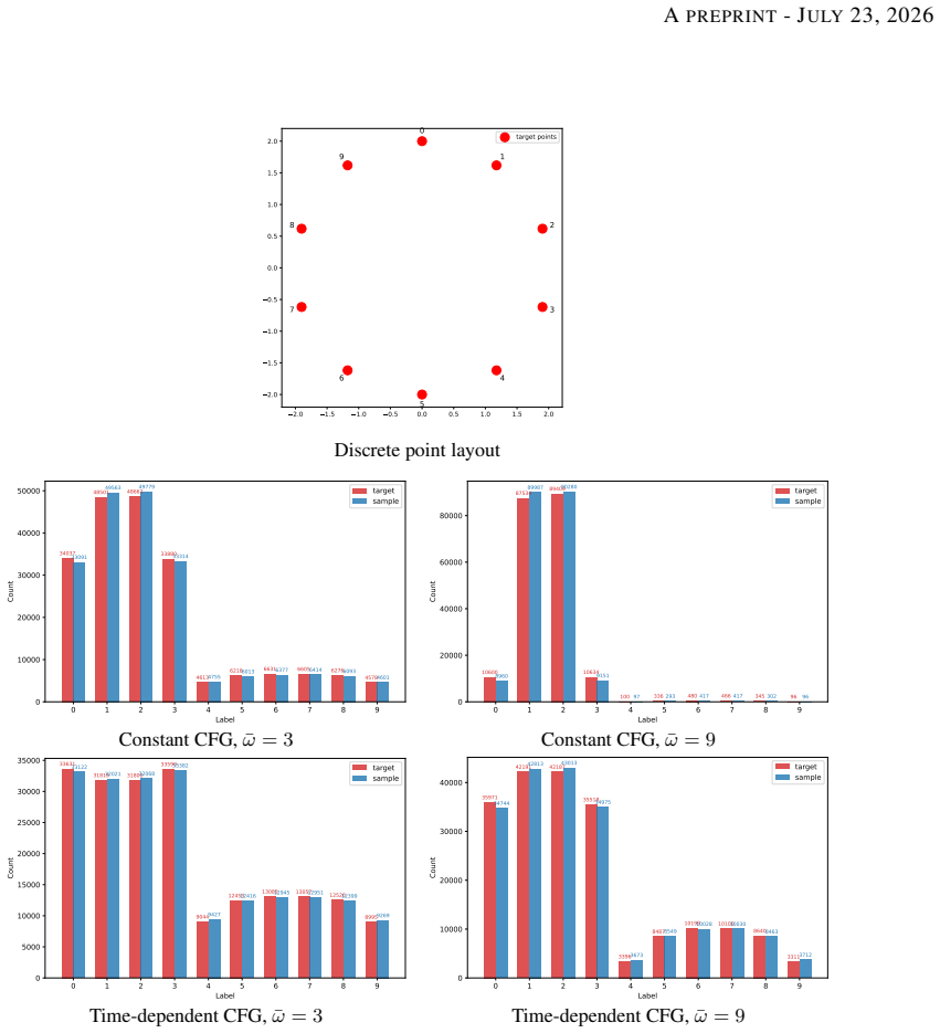
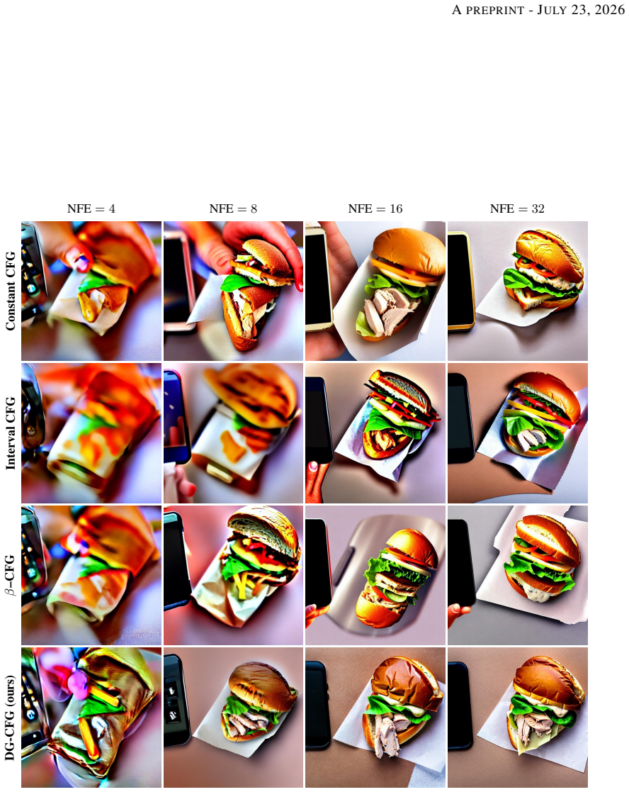
Summary. The paper derives an exact path-integral representation of the distribution induced by deterministic classifier-free guidance (CFG) in the probability-flow ODE framework. For constant guidance, Theorem 4.3 expresses the sampled density as the conditional marginal p_{t0} times an exponential path integral involving the score discrepancy; for time-dependent guidance, Theorem 4.4 gives the analogous formula with the schedule entering through ω(t)-1. The paper then uses the VPSDE specialization g^2=β(t) to motivate a schedule, DG-CFG, of the form ω(t)=1+C(ω̄-1)(1-ᾱ_t)√ᾱ_t/β(t), intended to balance the per-timestep path-integral contribution. The theoretical formulas are verified on a ten-point circle mixture with analytic scores, and DG-CFG is evaluated against constant, interval, and β-schedules on Stable Diffusion 1.5 across guidance strengths, ablations, and NFE budgets.
Significance. If the theorems are correct, the paper gives a substantive theoretical characterization of deterministic CFG, going beyond the common product-distribution heuristic and providing a principled language for time-dependent guidance. The derivation is self-contained, with explicit regularity assumptions, and the toy-model verification reports TV errors around 1-2%, which is a genuine strength. The proof strategy is transparent and the path-integral representation is non-circular in the sense that the characteristic flow depends only on the known score fields p and q, not on the unknown transported density. However, the paper's practical contribution, the DG-CFG schedule, is only loosely connected to the exact formula: the geometry-dependent term A_s = ΔL_s + ∇L_s·∇log p_s is not measured or modeled, and the SD1.5 evaluation consists of single-run point estimates without error bars. The central theoretical claim is defensible, but the schedule-design claim and the empirical validation need additional support.
major comments (4)
- [Sections 5.1–5.2, Eqs. (26)–(28)] The derivation of DG-CFG treats β(s) as the only schedule-dependent factor, but the exact path integral (24) has integrand β(s)(ω(s)-1)[ΔL_s + ∇L_s·∇log p_s]. The claim that constant CFG overweights high-noise by two orders of magnitude, and the Step-1 time-balancing construction, are valid only if the geometry factor A_s is roughly uniform or at least does not anti-correlate with β. The paper never measures A_s or reports time-resolved values of the integrand, and the Limitations paragraph concedes that geometric structure is not optimized. This is load-bearing because DG-CFG is presented as derived from the path-integral representation. Please either report time-resolved A_s on the toy model or on real SD1.5 trajectories, or explicitly reframe Step 1 as a heuristic based on the known β coefficient alone rather than as a consequence of the path-integral formula.
- [Section 6.2, Tables 2–5] All Stable Diffusion results are single-run point estimates on N=1,000 prompts (with Div computed on 100 prompts). No error bars, multiple seeds, or significance tests are reported. Several claimed improvements are small relative to plausible sampling noise, e.g., at ω̄=7 in Table 2 the FID difference is 67.67 vs. 67.87 and the IR difference is −0.115 vs. −0.103. The fixed-quality NFE conclusions in Table 5 also rest on differences of 2–4 steps. Without uncertainty quantification, the practical claims that DG-CFG improves the diversity–fidelity trade-off and reduces sampling cost are not established. Please add repeated runs or bootstrap confidence intervals, and state how many seeds were used.
- [Section 6.1, end of §6.1.1] The toy-model verification validates Theorems 4.3 and 4.4 for the schedule ω(t)=1+C(ω̄-1)√ᾱ_t/β(t), but explicitly omits the (1−ᾱ_t) factor that is part of the final DG-CFG schedule in Eq. (27). Thus the toy experiment does not validate the full DG-CFG schedule, nor does it test the claim that compensating only β(t) balances the true path-integral weight. The paper's statement that the toy 'directly validates the distributional formulas' is accurate, but the schedule-design mechanism remains unverified. Please either verify the final DG-CFG schedule against the predicted distribution in the toy model, or state clearly that the full schedule is a heuristic combination whose components are only partly motivated by the theorem.
- [Section 4.1, Theorems 4.3–4.4, Eqs. (20) and (24)] The simplified formulas used in the schedule-design section require the idealized terminal condition log p_T = log q_T. The paper explicitly acknowledges this, but the magnitude of the dropped boundary factor (p_T/q_T)^{ω(T)−1} is not quantified for realistic samplers, where p_T and q_T are close but not identical. For DG-CFG this is less concerning because ω(T)=1 by construction, but for constant CFG the boundary factor could be non-negligible. Please quantify the sensitivity of the prediction to this assumption, for instance by measuring the p_T/q_T ratio in the toy model or by reporting an error bound in terms of the terminal log-density difference.
minor comments (5)
- [Notation throughout] The symbol ω is used both for a constant guidance strength and for a time-dependent function. The notation is clear in context, but in Section 5 it becomes easy to confuse ω̄ and ω(t); a distinct symbol for the constant baseline would improve readability.
- [Eq. (27) and text after it] The sentence 'The resulting factor (1−ᾱ_t)√ᾱ_t/β(t) vanishes near both endpoints' is only approximate for t0>0: near t=t0, 1−ᾱ_t is small but not exactly zero unless t0=0. This is a minor wording issue, but it matters because the schedule is defined on [t0,T].
- [Section 6.2.1] The setup says 'randomly select N=1,000 prompt–image pairs' but then generates one image per prompt; the wording 'prompt–image pairs' is misleading. It should say '1,000 prompts' with one generated image each.
- [Appendix B] The theoretical label computation uses Nepoch=1000 perturbations per support point, but no random seed is reported. For reproducibility, please state the seed used in the toy experiments.
- [References] Reference [32], 'Classifier-free guidance with adaptive scaling', appears to be a preprint without a venue or year in the citation; please complete the bibliographic information.
Circularity Check
No significant circularity: the distribution theorems are self-contained, the toy check is a genuine prediction, and the schedule heuristics are flagged engineering choices rather than fitted outputs.
full rationale
The paper's central derivation (Theorems 4.2, 4.3, 4.4) is a self-contained Fokker-Planck/characteristic calculation from the guided probability flow ODE, with explicitly stated regularity and terminal-condition assumptions. The terminal condition log p_T = log q_T is presented as an idealized large-T approximation, not as an input that already encodes the conclusion. The toy-model verification compares actual DDIM samples against path-integral predictions computed with a finer discretization and no fitted parameters; the constants C are fixed by integral normalization of the guidance budget, not by matching output metrics, so this is a genuine prediction rather than a fitted input relabeled as validation. The DG-CFG schedule (Eq. 27) introduces multiplicative factors 1/beta, sqrt(alpha-bar), and 1-alpha-bar that are motivated by the structure of the path-integral exponent, but the paper itself acknowledges in Limitations that it 'does not explicitly optimize the geometric structure of the score discrepancy.' This is an under-supported engineering simplification or correctness gap, not a self-referential reduction: no claim in the derivation chain is justified by citing the present authors' prior work, and no load-bearing argument reduces to its own inputs by definition. The observed empirical gains are therefore not a consequence of circular reasoning, though the schedule's mechanism is less strongly established than its distributional formulas.
Axiom & Free-Parameter Ledger
axioms (4)
- domain assumption Forward marginals p_t, q_t are C^{1,2}, positive, solve the Fokker-Planck equation, and satisfy integrability and boundary-decay conditions (Assumption 4.1).
- domain assumption Idealized terminal condition log p_T = log q_T for all x (Section 4.1).
- domain assumption Score-approximation error in neural networks is amplified as 1/σ_t^2 near t0 (Section 5.2, Step 3).
- ad hoc to paper The geometry-dependent integrand ΔL_s + ∇L_s·∇log p_s can be treated as approximately uniform or subdominant for schedule design (Section 5; acknowledged in Limitations).
read the original abstract
Classifier-free guidance (CFG) is the default mechanism for conditional generation in diffusion models, but the distribution sampled by its deterministic guided dynamics is not captured by the usual product-distribution heuristic $p_0^\omega q_0^{1-\omega}$. We analyze CFG through the probability flow ODE and derive exact analytic path-integral representations of the induced distributions for both constant and time-dependent guidance. The resulting formulas show that CFG modifies $p_{t_0}$ by an exponential path-integral correction, and that a time-dependent schedule enters this correction through the weight $\omega(t)-1$. This characterization explains how score discrepancies accumulate along sampling trajectories and motivates Distribution-Guided CFG (DG-CFG), a schedule that balances timestep contributions while accounting for signal strength and low-noise score-error amplification. A toy model with analytic scores closely verifies the predicted distributions. On Stable Diffusion~1.5, DG-CFG improves generation and yields a stronger diversity--fidelity trade-off across guidance strengths, with especially clear gains when strong guidance causes saturation and quality degradation in constant and heuristic schedules. Across NFE budgets, DG-CFG reaches fixed image-quality targets with fewer sampling steps, reducing the sampling cost needed to achieve target metrics.
Figures


Reference graph
Works this paper leans on
-
[1]
Deep unsupervised learning using nonequilibrium thermodynamics
Jascha Sohl-Dickstein, Eric Weiss, Niru Maheswaranathan, and Surya Ganguli. Deep unsupervised learning using nonequilibrium thermodynamics. InInternational conference on machine learning, pages 2256–2265. pmlr, 2015
2015
-
[2]
Denoising diffusion probabilistic models.Advances in neural information processing systems, 33:6840–6851, 2020
Jonathan Ho, Ajay Jain, and Pieter Abbeel. Denoising diffusion probabilistic models.Advances in neural information processing systems, 33:6840–6851, 2020
2020
-
[3]
Score- based generative modeling through stochastic differential equations
Yang Song, Jascha Sohl-Dickstein, Diederik P Kingma, Abhishek Kumar, Stefano Ermon, and Ben Poole. Score- based generative modeling through stochastic differential equations. InInternational Conference on Learning Representations, 2021
2021
-
[4]
Diffusion models beat gans on image synthesis.Advances in neural information processing systems, 34:8780–8794, 2021
Prafulla Dhariwal and Alexander Nichol. Diffusion models beat gans on image synthesis.Advances in neural information processing systems, 34:8780–8794, 2021
2021
-
[5]
High-resolution image synthesis with latent diffusion models
Robin Rombach, Andreas Blattmann, Dominik Lorenz, Patrick Esser, and Björn Ommer. High-resolution image synthesis with latent diffusion models. InProceedings of the IEEE/CVF conference on computer vision and pattern recognition, pages 10684–10695, 2022
2022
-
[6]
Video diffusion models.Advances in neural information processing systems, 35:8633–8646, 2022
Jonathan Ho, Tim Salimans, Alexey Gritsenko, William Chan, Mohammad Norouzi, and David J Fleet. Video diffusion models.Advances in neural information processing systems, 35:8633–8646, 2022
2022
-
[7]
Diffwave: A versatile diffusion model for audio synthesis
Zhifeng Kong, Wei Ping, Jiaji Huang, Kexin Zhao, and Bryan Catanzaro. Diffwave: A versatile diffusion model for audio synthesis. InInternational Conference on Learning Representations, 2021
2021
-
[8]
Geodiff: A geometric diffusion model for molecular conformation generation
Minkai Xu, Lantao Yu, Yang Song, Chence Shi, Stefano Ermon, and Jian Tang. Geodiff: A geometric diffusion model for molecular conformation generation. InInternational Conference on Learning Representations, 2022
2022
-
[9]
Classifier-free diffusion guidance
Jonathan Ho and Tim Salimans. Classifier-free diffusion guidance. InNeurIPS 2021 Workshop on Deep Generative Models and Downstream Applications, 2021
2021
-
[10]
Photorealistic text-to-image diffusion models with deep language understanding.Advances in neural information processing systems, 35:36479–36494, 2022
Chitwan Saharia, William Chan, Saurabh Saxena, Lala Li, Jay Whang, Emily L Denton, Kamyar Ghasemipour, Raphael Gontijo Lopes, Burcu Karagol Ayan, Tim Salimans, et al. Photorealistic text-to-image diffusion models with deep language understanding.Advances in neural information processing systems, 35:36479–36494, 2022. 16 APREPRINT- JULY23, 2026
2022
-
[11]
Aditya Ramesh, Prafulla Dhariwal, Alex Nichol, Casey Chu, and Mark Chen. Hierarchical text-conditional image generation with clip latents.arXiv preprint arXiv:2204.06125, 1(2):3, 2022
Pith/arXiv arXiv 2022
-
[12]
Yogesh Balaji, Seungjun Nah, Xun Huang, Arash Vahdat, Jiaming Song, Qinsheng Zhang, Karsten Kreis, Miika Aittala, Timo Aila, Samuli Laine, et al. ediff-i: Text-to-image diffusion models with an ensemble of expert denoisers.arXiv preprint arXiv:2211.01324, 2022
Pith/arXiv arXiv 2022
-
[13]
Haohe Liu, Zehua Chen, Yi Yuan, Xinhao Mei, Xubo Liu, Danilo Mandic, Wenwu Wang, and Mark D Plumbley. Audioldm: Text-to-audio generation with latent diffusion models.arXiv preprint arXiv:2301.12503, 2023
Pith/arXiv arXiv 2023
-
[14]
Barron, and Ben Mildenhall
Ben Poole, Ajay Jain, Jonathan T. Barron, and Ben Mildenhall. Dreamfusion: Text-to-3d using 2d diffusion. In The Eleventh International Conference on Learning Representations, 2023
2023
-
[15]
Reverse-time diffusion equation models.Stochastic Processes and their Applications, 12(3):313–326, 1982
Brian DO Anderson. Reverse-time diffusion equation models.Stochastic Processes and their Applications, 12(3):313–326, 1982
1982
-
[16]
Denoising diffusion implicit models
Jiaming Song, Chenlin Meng, and Stefano Ermon. Denoising diffusion implicit models. InInternational Conference on Learning Representations, 2021
2021
-
[17]
Elucidating the design space of diffusion-based generative models.Advances in neural information processing systems, 35:26565–26577, 2022
Tero Karras, Miika Aittala, Timo Aila, and Samuli Laine. Elucidating the design space of diffusion-based generative models.Advances in neural information processing systems, 35:26565–26577, 2022
2022
-
[18]
Estimation of non-normalized statistical models by score matching.Journal of Machine Learning Research, 6(4), 2005
Aapo Hyvärinen and Peter Dayan. Estimation of non-normalized statistical models by score matching.Journal of Machine Learning Research, 6(4), 2005
2005
-
[19]
A connection between score matching and denoising autoencoders.Neural computation, 23(7):1661–1674, 2011
Pascal Vincent. A connection between score matching and denoising autoencoders.Neural computation, 23(7):1661–1674, 2011
2011
-
[20]
Improved denoising diffusion probabilistic models
Alexander Quinn Nichol and Prafulla Dhariwal. Improved denoising diffusion probabilistic models. InInterna- tional conference on machine learning, pages 8162–8171. PMLR, 2021
2021
-
[21]
Progressive distillation for fast sampling of diffusion models
Tim Salimans and Jonathan Ho. Progressive distillation for fast sampling of diffusion models. InInternational Conference on Learning Representations, 2022
2022
-
[22]
Dpm-solver: A fast ode solver for diffusion probabilistic model sampling in around 10 steps.Advances in neural information processing systems, 35:5775–5787, 2022
Cheng Lu, Yuhao Zhou, Fan Bao, Jianfei Chen, Chongxuan Li, and Jun Zhu. Dpm-solver: A fast ode solver for diffusion probabilistic model sampling in around 10 steps.Advances in neural information processing systems, 35:5775–5787, 2022
2022
-
[23]
Score-based generative modeling in latent space.Advances in neural information processing systems, 34:11287–11302, 2021
Arash Vahdat, Karsten Kreis, and Jan Kautz. Score-based generative modeling in latent space.Advances in neural information processing systems, 34:11287–11302, 2021
2021
-
[24]
Cfg++: Manifold-constrained classifier free guidance for diffusion models
Hyungjin Chung, Jeongsol Kim, Geon Yeong Park, Hyelin Nam, and Jong Chul Ye. Cfg++: Manifold-constrained classifier free guidance for diffusion models. InInternational Conference on Learning Representations, volume 2025, pages 30824–30850, 2025
2025
-
[25]
Guiding a diffusion model with a bad version of itself.Advances in Neural Information Processing Systems, 37:52996–53021, 2024
Tero Karras, Miika Aittala, Tuomas Kynkäänniemi, Jaakko Lehtinen, Timo Aila, and Samuli Laine. Guiding a diffusion model with a bad version of itself.Advances in Neural Information Processing Systems, 37:52996–53021, 2024
2024
-
[26]
Eliminating oversaturation and artifacts of high guidance scales in diffusion models
Seyedmorteza Sadat, Otmar Hilliges, and Romann M Weber. Eliminating oversaturation and artifacts of high guidance scales in diffusion models. InThe Thirteenth International Conference on Learning Representations, 2024
2024
-
[27]
Classifier-free guidance is a predictor-corrector.arXiv preprint arXiv:2408.09000, 2024
Arwen Bradley and Preetum Nakkiran. Classifier-free guidance is a predictor-corrector.arXiv preprint arXiv:2408.09000, 2024
Pith/arXiv arXiv 2024
-
[28]
Understanding classifier-free guidance: High-dimensional theory and non-linear generalizations.arXiv e-prints, pages arXiv–2502, 2025
Krunoslav Lehman Pavasovic, Jakob Verbeek, Giulio Biroli, and Marc Mezard. Understanding classifier-free guidance: High-dimensional theory and non-linear generalizations.arXiv e-prints, pages arXiv–2502, 2025
2025
-
[29]
Stage-wise dynamics of classifier-free guidance in diffusion models
Cheng Jin, Qitan Shi, and Yuantao Gu. Stage-wise dynamics of classifier-free guidance in diffusion models. In The Fourteenth International Conference on Learning Representations, 2026
2026
-
[30]
Feynman-kac correctors in diffusion: Annealing, guidance, and product of experts
Marta Skreta, Tara Akhound-Sadegh, Viktor Ohanesian, Roberto Bondesan, Alan Aspuru-Guzik, Arnaud Doucet, Rob Brekelmans, Alexander Tong, and Kirill Neklyudov. Feynman-kac correctors in diffusion: Annealing, guidance, and product of experts. InForty-second International Conference on Machine Learning, 2025
2025
-
[31]
Peipei Gao, Gang Zeng, and Yanting Ma. C2fg: A more efficient training-free classifier-free guidance for text-to-image diffusion models.arXiv preprint arXiv:2601.01412, 2026
arXiv 2026
-
[32]
Classifier-free guidance with adaptive scaling
Dawid Malarz, Artur Kasymov, Maciej Zi˛ eba, Jacek Tabor, and Przemysław Spurek. Classifier-free guidance with adaptive scaling. 2025. 17 APREPRINT- JULY23, 2026
2025
-
[33]
Applying guidance in a limited interval improves sample and distribution quality in diffusion models.Advances in Neural Information Processing Systems, 37:122458–122483, 2024
Tuomas Kynkäänniemi, Miika Aittala, Tero Karras, Samuli Laine, Timo Aila, and Jaakko Lehtinen. Applying guidance in a limited interval improves sample and distribution quality in diffusion models.Advances in Neural Information Processing Systems, 37:122458–122483, 2024
2024
-
[34]
Microsoft coco: Common objects in context
Tsung-Yi Lin, Michael Maire, Serge Belongie, James Hays, Pietro Perona, Deva Ramanan, Piotr Dollár, and C Lawrence Zitnick. Microsoft coco: Common objects in context. InEuropean conference on computer vision, pages 740–755. Springer, 2014
2014
-
[35]
Gans trained by a two time-scale update rule converge to a local nash equilibrium.Advances in neural information processing systems, 30, 2017
Martin Heusel, Hubert Ramsauer, Thomas Unterthiner, Bernhard Nessler, and Sepp Hochreiter. Gans trained by a two time-scale update rule converge to a local nash equilibrium.Advances in neural information processing systems, 30, 2017
2017
-
[36]
Learning transferable visual models from natural language supervision
Alec Radford, Jong Wook Kim, Chris Hallacy, Aditya Ramesh, Gabriel Goh, Sandhini Agarwal, Girish Sastry, Amanda Askell, Pamela Mishkin, Jack Clark, et al. Learning transferable visual models from natural language supervision. InInternational conference on machine learning, pages 8748–8763. PmLR, 2021
2021
-
[37]
The vendi score: A diversity evaluation metric for machine learning
Dan Friedman and Adji Bousso Dieng. The vendi score: A diversity evaluation metric for machine learning. Transactions on Machine Learning Research, 2023. A Proofs of Main Results This appendix gives the proofs of the three main theorems in Section 4. The arguments are organized by their logical dependence: we first derive the Fokker–Planck equation for th...
2023
discussion (0)
Sign in with ORCID, Apple, or X to comment. Anyone can read and Pith papers without signing in.