REVIEW 4 major objections 7 minor 72 references
Pulsar-timing searches for ultralight dark matter must use finite spatial correlations, not the fully correlated or uncorrelated limits, across the PTA mass range.
Reviewed by Pith at T0; open to challenge. T0 means a machine referee read the full paper against a public rubric. the ladder, T0–T4 →
T0 review · grok-4.5
2026-07-31 06:07 UTC pith:VGHZLISC
load-bearing objection Solid methods paper that finally turns finite ULDM spatial correlations into a usable PTA analysis; limiting priors really do bias quadratic limits by up to ~1 dex on mocks. the 4 major comments →
Correlated signals of ultralight scalar dark matter in pulsar timing
The pith
A machine-rendered reading of the paper's core claim, the machinery that carries it, and where it could break.
Core claim
A self-consistent PTA analysis that models ultralight scalar dark matter as a Gaussian random field with finite spatial correlations supplies a continuous amplitude prior between the fully correlated and fully uncorrelated limits; on mock data the limiting priors bias 95 percent upper limits by up to ~0.3 dex (linear) and nearly 1 dex (quadratic), while blinded injections recover the true mass and amplitudes inside the posterior support.
What carries the argument
The augmented latent-field prior: pulsar distances set only the slow correlation magnitudes R_IJ, retarded-time phases are treated as independent uniform nuisances, and the resulting distance-marginalized joint amplitude distribution is represented by a mass-by-mass normalizing-flow surrogate that is sampled inside the ordinary PTA likelihood.
Load-bearing premise
The method assumes that current pulsar-distance uncertainties leave the rapid oscillation phases completely free, so those phases can be randomized independently of distance without distorting the amplitude prior that actually carries the correlation information.
What would settle it
Run the finite-correlation pipeline and both limiting priors on the same real PTA data set (or on an ensemble of mocks with known injected masses spanning 10^-24–10^-20 eV) and check whether the recovered 95 percent amplitude limits differ by the predicted O(0.1–1) dex in the intermediate-mass window while blinded recovery still places the true mass and amplitudes inside the posterior support.
If this is right
- Published PTA bounds that assumed a single limiting prior across the full mass range should be re-derived with the finite-correlation prior before they are treated as definitive.
- Projected sensitivities for next-generation PTAs must quote the continuous-correlation curve rather than the more optimistic or pessimistic limiting envelope.
- The same latent-field construction applies unchanged to the quadratic gravitational signal, so metric-only and SM-coupled searches can share one amplitude prior.
- Vector (dark-photon) ULDM searches can reuse the pipeline once the latent prior is enlarged to a vector-valued field.
- Mass-by-mass evidence-weighted scans become the practical route to joint mass–amplitude posteriors when the number of resolvable Fourier bins is large.
Where Pith is reading between the lines
- Once real-data re-analyses appear, tension or agreement between PTA limits and laboratory clock or equivalence-principle bounds on the same couplings will become sharper because the intermediate-mass systematics will be under control.
- The normalizing-flow compression of a high-dimensional distance-marginalized prior is a reusable template for any PTA signal whose spatial coherence length is comparable to array baselines.
- If future distance measurements tighten below the Compton scale at the lowest masses, the phase-augmentation step will have to be revisited or replaced by joint sampling of distance and phase.
Editorial analysis
A structured set of objections, weighed in public.
Referee Report
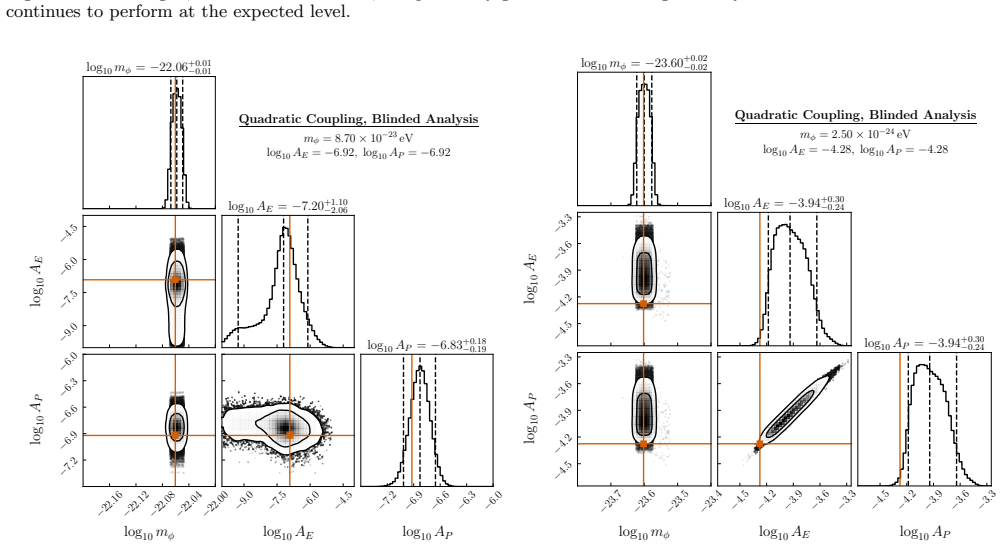
Summary. The manuscript develops a PTA analysis of the ULDM fast mode that retains finite spatial correlations of the underlying Gaussian field. The authors derive the retarded-time covariance, convert it into a joint latent amplitude–phase prior, incorporate pulsar-distance uncertainty through an augmented prior with independent effective phases, and represent the resulting distance-marginalized amplitude distribution with mass-specific neural spline flows. The same latent construction is used for linearly coupled, quadratically coupled, and universal gravitational signals. Mock 30-pulsar analyses include null tests, unblinded injections, and evidence-weighted blinded mass scans. The null tests indicate that the fully correlated and fully uncorrelated limiting priors can shift 95% amplitude limits by up to about 0.3 dex for a linear response and nearly 1 dex for a quadratic response.
Significance. This is a substantial methodological advance because the correlated-to-uncorrelated transition lies directly within the PTA-sensitive mass range, and existing limits can depend on which limiting prior is imposed. The covariance derivation is clearly presented, Appendix C strengthens the Gaussianity result for the slow mode, and Appendix G transparently derives the factorized augmented prior and recovers both standard Rayleigh-prior limits. The flow implementation and blinded end-to-end tests make the method practically credible. If the augmented-prior approximation and surrogate accuracy are quantified, the framework should become the appropriate default for scalar-ULDM PTA searches and is naturally extensible to other ULDM signals.
major comments (4)
- [Sec. IV C, Eq. (60); Appendix G] The augmented prior replaces the exact link ψ_I=mφx_I with independent uniform phases. Appendix G proves factorization only after that replacement; it does not establish proximity to the exact prior in Eq. (60). The phase-rotation argument does protect the distance-marginalized amplitude law π(A|mφ), so the concern is not that marginal itself. However, the exact model retains amplitude–phase and phase–phase correlations that can enter the latent-marginalized likelihood and hence the reported upper limits. The wrapping argument is plausible but unquantified: at 10^-24 eV, mφ^-1≃6.4 pc while J0030+0451 has σ_x=3.6 pc. Please either derive an error bound involving wrapped-phase nonuniformity and the distance-induced variation of R_IJ, or compare against the exact linked-phase model by importance reweighting, a restricted exact sampler, or exact-mixture injections at representative low and t
- [Sec. IV D, Fig. 3, Appendix H] The trained flow is the prior actually used in inference, but its validation is visual, restricted to the first three amplitudes, and shown at only two endpoint masses. This does not establish all-pair, tail, or intermediate-mass fidelity at the accuracy needed to attribute 0.3–1 dex posterior shifts to physical correlation structure rather than surrogate error. Please add held-out quantitative diagnostics (log-density or density-ratio performance, pairwise-correlation and tail calibration, and training-set-size convergence), and validate the inferred posterior or upper limit at a few representative masses against either the explicit augmented sampler described in Sec. IV E or an independently trained architecture.
- [Sec. V C, Figs. 4–6] The quantitative comparisons in Figs. 4–6, including the stated factor-of-two and nearly-order-of-magnitude shifts, are based on one null realization. Comparing models on the same realization cancels some noise, but it does not establish that these shifts are systematic prior effects rather than realization fluctuations. Since these numbers are central to the abstract and conclusions, please repeat the null comparison for several background realizations at selected correlated, transition, and uncorrelated masses and report the mean and scatter of Δlog10 Aφ; alternatively, explicitly downgrade the numerical shifts to properties of one illustrative realization. The same qualification applies to the density translation in Fig. 6.
- [Sec. V E, Eqs. (67)–(69)] The adaptive grid in Eq. (67) is nonuniform, but Eq. (69) does not define the prior weights π(m_i). An evidence-weighted mass posterior requires the integrated log-uniform prior probability associated with each grid cell, not an equal weight or the point density π(m_i); otherwise the nonuniform sampling itself biases the inferred mass posterior. Please specify the cell boundaries and weights used in Figs. 9–10 and 13–14, and recalculate those figures if volume weighting was not already included.
minor comments (7)
- [Sec. V D, Figs. 7 and 12] The text generally describes the injections as successfully recovered, but Fig. 7 notes that the injected γ_GW lies slightly outside the central 90% interval, and in the right panel of Fig. 12 the injected Aφ is also slightly outside that interval. These are not individually alarming, but the recovery language should be made more precise and accompanied by a compact coverage summary across all injection parameters.
- [Sec. III A, Fig. 2] The numerical check of the monochromatic approximation uses one geometry and retarded-time separation and the plotted range appears to stop near 10^-22 eV, whereas the analyses extend to 10^-20 eV. Please either extend the comparison over the full mass range and several baselines/times or provide a short absolute-error bound supporting Eq. (40) throughout the analysis domain.
- [Sec. V B, Eq. (66)] The mass-dependent bounds in Eq. (66) were chosen using preliminary null behavior. The prior-percentile diagnostic in Figs. 4–5 is useful, but a brief sensitivity check to a broader and narrower A_max would further demonstrate that the quoted 95% limits are not controlled by the adopted bounds.
- [Secs. II C and V C] The finite-correlation transition depends on the assumed isotropic Maxwell–Boltzmann halo and fixed v0=155 km/s. A sentence quantifying how plausible v0 variations shift the transition mass, or explicitly identifying this as a fixed-halo projection, would help readers interpret Figs. 4–6.
- [Sec. V A] The manuscript says a modified version of PTA Replicator was used, but links only the upstream package. Release of the modification, analysis scripts, flow-training code, and either trained flows or regeneration instructions would substantially improve reproducibility.
- [Fig. 3] Please state the probability levels represented by the blue and green contours in Fig. 3. This is especially useful because the figure currently supplies the main visual check of the flow surrogate.
- [Appendix K] The statement that the Gaussian-process covariance becomes numerically ill-conditioned would be more useful if accompanied by a representative condition number or a criterion for where the instability occurs.
Circularity Check
No significant circularity: finite-correlation prior is derived from the Gaussian field covariance and validated on mocks without reducing predictions to fitted inputs.
full rationale
The paper's central construction is a latent amplitude prior obtained from the ULDM two-point function (Eqs. 37–50), with distance marginalization via an augmented generative model and a normalizing-flow surrogate. That prior is an input modeling choice, not a fitted prediction of the mock limits. The reported O(0.1–1 dex) shifts versus fully correlated/uncorrelated analyses are differences between three analysis priors applied to the same synthetic data, not quantities forced by construction from a fit. Blinded injection recovery tests unknown injected masses/amplitudes against the pipeline; recovery within posterior support is ordinary method validation, not circular. Self-citations to the authors' prior correlation theory ([35,36]) supply background formalism; the end-to-end PTA likelihood, flow prior, and mock results are developed and checked in this work. The augmented phase–distance factorization (Sec. IV C, App. G) is an approximation whose fidelity is a correctness question, not a definitional loop. No step reduces a claimed first-principles result to its own inputs by construction.
Axiom & Free-Parameter Ledger
free parameters (4)
- A_max(m_φ), A_min(m_φ) mass-dependent log-uniform amplitude prior bounds =
A_max = [1e-5 + 0.1 (m_φ/1e-24 eV)^{-3}] s; A_min = 1e-5 A_max
- Normalizing-flow architecture hyperparameters =
as stated in App. H
- Mock SGWB amplitude and index =
A_GW=6.4e-15, γ_GW=3.2
- Local DM density ρ_φ and velocity dispersion v_0 =
ρ_φ≃0.4 GeV/cm³, v_0≈155 km/s
axioms (6)
- domain assumption ULDM is a Gaussian random field from Rayleigh amplitudes and random phases (or equivalent Gaussian quadratures) with isotropic Maxwell-Boltzmann velocities.
- domain assumption Monochromatic approximation ω_v → m_φ is accurate enough that absolute covariance error remains negligible across the PTA mass range.
- ad hoc to paper After treating effective distance phases as i.i.d. uniform nuisances, physical phases α_I are uniform and independent of amplitudes, so all spatial information sits in π(A|m_φ).
- ad hoc to paper A mass-specific neural spline flow trained on augmented generative samples is a faithful surrogate for the distance-marginalized amplitude prior.
- domain assumption Quadratic slow mode is exactly Gaussian in the continuum limit and can be deferred; analysis restricts to the fast mode.
- domain assumption Standard PTA background model: white noise + uncorrelated red noise + Hellings–Downs SGWB, with timing-model analytic marginalization.
invented entities (2)
-
Augmented latent-field prior with independent nuisance phases ψ_I
no independent evidence
-
Normalizing-flow surrogate π_flow(A|m_φ) for latent ULDM amplitudes
no independent evidence
read the original abstract
Pulsar timing arrays (PTAs) are sensitive to ultralight dark matter (ULDM) in the $10^{-24}$-$10^{-20}\,\mathrm{eV}$ mass range, with existing datasets already probing otherwise open parameter space and future PTAs promising substantial improvements in reach. Thus far, however, PTA searches for ULDM have typically been formulated using limiting descriptions. Analyses are performed in either the fully correlated limit, in which the local ULDM amplitude is shared across the array, or the fully uncorrelated limit, in which each pulsar has an independent local amplitude. Because the transition between these regimes occurs within the PTA-sensitive mass range, projected sensitivities and data-derived constraints can depend on which limiting description is assumed. For the first time, we develop a self-consistent analysis that treats the ULDM field as a Gaussian random field with finite spatial correlations, allowing the amplitude prior used in PTA signal models to interpolate continuously between the fully correlated and fully uncorrelated limits. We apply the framework to both linearly and quadratically coupled scalar ULDM, the latter including the universal gravitational signal sourced by the oscillating ULDM pressure. Pulsar-distance uncertainties are incorporated through an augmented latent-field prior, and the resulting distance-marginalized latent-amplitude distribution is represented with a normalizing-flow surrogate. We validate the method on mock PTA datasets, including blinded signal injection tests.
Figures


Reference graph
Works this paper leans on
-
[1]
PX,” or from dispersion measures using the NE2001 free-electron den- sity model, indicated by “DM
Its pulsar-timing phenomenology was studied in Ref. [29], which argued that it is approx- imately Gaussian. Here we show that in the continuum limit it is exactly Gaussian, so that it may be treated as an ordinary stationary Gaussian process specified en- tirely by its power spectrum. We continue to work with the unit-normalized contin- uum quadratures in...
1902
-
[2]
Latent amplitude-phase statistics For a specified ULDM massm ϕ, the monochromatic retarded-time field at locationImay be written as ˆϕI (t) = ˆCI cos(mϕt) + ˆSI sin(mϕt),(G1) with{( ˆCI , ˆSI )}jointly Gaussian distributed according to Eq. (50). It is convenient to combine these variables into the complex amplitudes ˆzI ≡ ˆCI +i ˆSI =A I eiαI .(G2) In ter...
-
[3]
Relation to previous analyses The augmented formulation also makes it straightfor- ward to recover the limiting signal models used in previ- ous PTA analyses of ULDM. In the fully correlated limit,ℓ→ ∞, the correlation- envelope matrix approaches RIJ →1,R→11 T .(G12) The rotated latent vector ˆwtherefore becomes rank one, so there exists a single proper c...
2048
-
[4]
Signal construction For the fixed coupling-ratio parametrization, starting from Eq. (26), we write the induced timing residual for pulsarIas rI (t) =A ϕ [CI cos(mϕt) +S I sin(mϕt)],(K1) where the residual-level cosine-sine coefficients are CI ≡w E ˆC0 +w P ˆCI , S I ≡w E ˆS0 +w P ˆSI .(K2) HereI, J≥1 label pulsars, while the index 0 denotes Earth. Using E...
-
[5]
Gaussian-process likelihood At fixed pulsar distances and effective phases, the Gaussian-process likelihood is obtained by adding the ULDM signal covariance in Eq. (K12) to the background covariance, Σtot =Σ bkg +Σ ϕ.(K13) For a PTA residual vectord PTA, the corresponding like- lihood is LGP(dPTA |θ bkg, Aϕ,{x I },{ψ I }) = 1 |2πΣtot|1/2 ×exp − 1 2 dT PTA...
-
[6]
New Horizons: Scalar and Vector Ultralight Dark Matter,
D. Antypaset al., “New Horizons: Scalar and Vector Ultralight Dark Matter,” (3, 2022) ,arXiv:2203.14915 [hep-ex]
arXiv 2022
-
[7]
Pulsar timing signal from ultralight scalar dark matter,
A. Khmelnitsky and V. Rubakov, “Pulsar timing signal from ultralight scalar dark matter,”JCAP02(2014) 019,arXiv:1309.5888 [astro-ph.CO]
Pith/arXiv arXiv 2014
-
[8]
The String dilaton and a least coupling principle,
T. Damour and A. M. Polyakov, “The String dilaton and a least coupling principle,”Nucl. Phys. B423 (1994) 532–558,arXiv:hep-th/9401069
Pith/arXiv arXiv 1994
-
[9]
Violations of the equivalence principle in a dilaton runaway scenario,
T. Damour, F. Piazza, and G. Veneziano, “Violations of the equivalence principle in a dilaton runaway scenario,” Phys. Rev. D66(2002) 046007,arXiv:hep-th/0205111
Pith/arXiv arXiv 2002
-
[10]
Dilatonic dark matter and its experimental detection,
Y. M. Cho and J. H. Kim, “Dilatonic dark matter and its experimental detection,”Phys. Rev. D79(2009) 023504,arXiv:0711.2858 [gr-qc]
Pith/arXiv arXiv 2009
-
[11]
Equivalence Principle Violations and Couplings of a Light Dilaton,
T. Damour and J. F. Donoghue, “Equivalence Principle Violations and Couplings of a Light Dilaton,”Phys. Rev. D82(2010) 084033,arXiv:1007.2792 [gr-qc]
Pith/arXiv arXiv 2010
-
[12]
Constraints on the variations of the fundamental couplings,
K. A. Olive, M. Pospelov, Y.-Z. Qian, A. Coc, M. Casse, and E. Vangioni-Flam, “Constraints on the variations of the fundamental couplings,”Phys. Rev. D 66(2002) 045022,arXiv:hep-ph/0205269
Pith/arXiv arXiv 2002
-
[13]
V. V. Flambaum, D. B. Leinweber, A. W. Thomas, and R. D. Young, “Limits on the temporal variation of the 32 fine structure constant, quark masses and strong interaction from quasar absorption spectra and atomic clock experiments,”Phys. Rev. D69(2004) 115006, arXiv:hep-ph/0402098
Pith/arXiv arXiv 2004
-
[14]
Phenomenology of the Equivalence Principle with Light Scalars,
T. Damour and J. F. Donoghue, “Phenomenology of the Equivalence Principle with Light Scalars,”Class. Quant. Grav.27(2010) 202001,arXiv:1007.2790 [gr-qc]
Pith/arXiv arXiv 2010
-
[15]
Search for ultralight scalar dark matter with atomic spectroscopy,
K. Van Tilburg, N. Leefer, L. Bougas, and D. Budker, “Search for ultralight scalar dark matter with atomic spectroscopy,”Phys. Rev. Lett.115no. 1, (2015) 011802,arXiv:1503.06886 [physics.atom-ph]
Pith/arXiv arXiv 2015
-
[16]
A. Hees, J. Gu´ ena, M. Abgrall, S. Bize, and P. Wolf, “Searching for an oscillating massive scalar field as a dark matter candidate using atomic hyperfine frequency comparisons,”Phys. Rev. Lett.117no. 6, (2016) 061301,arXiv:1604.08514 [gr-qc]
Pith/arXiv arXiv 2016
-
[17]
J. Berg´ e, P. Brax, G. M´ etris, M. Pernot-Borr` as, P. Touboul, and J.-P. Uzan, “MICROSCOPE Mission: First Constraints on the Violation of the Weak Equivalence Principle by a Light Scalar Dilaton,”Phys. Rev. Lett.120no. 14, (2018) 141101, arXiv:1712.00483 [gr-qc]
Pith/arXiv arXiv 2018
-
[18]
Violation of the equivalence principle from light scalar dark matter,
A. Hees, O. Minazzoli, E. Savalle, Y. V. Stadnik, and P. Wolf, “Violation of the equivalence principle from light scalar dark matter,”Phys. Rev. D98no. 6, (2018) 064051,arXiv:1807.04512 [gr-qc]
Pith/arXiv arXiv 2018
-
[19]
New bounds on dark matter coupling from a global network of optical atomic clocks,
P. Wcis loet al., “New bounds on dark matter coupling from a global network of optical atomic clocks,”Sci. Adv.4no. 12, (2018) eaau4869,arXiv:1806.04762 [physics.atom-ph]
Pith/arXiv arXiv 2018
-
[20]
C. J. Kennedy, E. Oelker, J. M. Robinson, T. Bothwell, D. Kedar, W. R. Milner, G. E. Marti, A. Derevianko, and J. Ye, “Precision Metrology Meets Cosmology: Improved Constraints on Ultralight Dark Matter from Atom-Cavity Frequency Comparisons,”Phys. Rev. Lett. 125no. 20, (2020) 201302,arXiv:2008.08773 [physics.atom-ph]
Pith/arXiv arXiv 2020
-
[21]
H. Davoudiasl and P. B. Denton, “How fast can protons decay?,”Phys. Rev. D111no. 3, (2025) 035026, arXiv:2410.19045 [hep-ph]
Pith/arXiv arXiv 2025
-
[22]
Cosmological constraints on a dynamical electron mass,
J. D. Barrow and J. Magueijo, “Cosmological constraints on a dynamical electron mass,”Phys. Rev. D72(2005) 043521,arXiv:astro-ph/0503222
Pith/arXiv arXiv 2005
-
[23]
Can dark matter induce cosmological evolution of the fundamental constants of Nature?,
Y. V. Stadnik and V. V. Flambaum, “Can dark matter induce cosmological evolution of the fundamental constants of Nature?,”Phys. Rev. Lett.115no. 20, (2015) 201301,arXiv:1503.08540 [astro-ph.CO]
Pith/arXiv arXiv 2015
-
[24]
BBN constraints on universally-coupled ultralight scalar dark matter,
S. Sibiryakov, P. Sørensen, and T.-T. Yu, “BBN constraints on universally-coupled ultralight scalar dark matter,”JHEP12(2020) 075,arXiv:2006.04820 [hep-ph]
Pith/arXiv arXiv 2020
-
[25]
Constraints on ultralight scalar dark matter with quadratic couplings,
T. Bouley, P. Sørensen, and T.-T. Yu, “Constraints on ultralight scalar dark matter with quadratic couplings,” JHEP03(2023) 104,arXiv:2211.09826 [hep-ph]
Pith/arXiv arXiv 2023
-
[26]
Cosmology with varying fundamental constants from hyperlight, coupled scalars,
M. Baryakhtar, O. Simon, and Z. J. Weiner, “Cosmology with varying fundamental constants from hyperlight, coupled scalars,”Phys. Rev. D110no. 8, (2024) 083505,arXiv:2405.10358 [astro-ph.CO]
Pith/arXiv arXiv 2024
-
[27]
Searching for coupled, hyperlight scalars across cosmic history,
M. Baryakhtar, O. Simon, and Z. J. Weiner, “Searching for coupled, hyperlight scalars across cosmic history,” Phys. Rev. D111no. 11, (2025) 115026, arXiv:2502.04432 [hep-ph]
Pith/arXiv arXiv 2025
-
[28]
S. Ghosh, K. K. Boddy, and T.-T. Yu, “Early Universe Constraints on Variations in Fundamental Constants Induced by Ultralight Scalar Dark Matter,” (11, 2025) , arXiv:2511.14532 [astro-ph.CO]
arXiv 2025
-
[29]
Time variation of proton-electron mass ratio and fine structure constant with runaway dilaton,
T. Chiba, T. Kobayashi, M. Yamaguchi, and J. Yokoyama, “Time variation of proton-electron mass ratio and fine structure constant with runaway dilaton,” Phys. Rev. D75(2007) 043516,arXiv:hep-ph/0610027
Pith/arXiv arXiv 2007
-
[30]
Dark Matter Direct Detection with Accelerometers,
P. W. Graham, D. E. Kaplan, J. Mardon, S. Rajendran, and W. A. Terrano, “Dark Matter Direct Detection with Accelerometers,”Phys. Rev. D93no. 7, (2016) 075029,arXiv:1512.06165 [hep-ph]
Pith/arXiv arXiv 2016
-
[31]
Constraining fundamental constant variations from ultralight dark matter with pulsar timing arrays,
D. E. Kaplan, A. Mitridate, and T. Trickle, “Constraining fundamental constant variations from ultralight dark matter with pulsar timing arrays,”Phys. Rev. D106no. 3, (2022) 035032,arXiv:2205.06817 [hep-ph]
Pith/arXiv arXiv 2022
-
[32]
The NANOGrav 15 yr Data Set: Search for Signals from New Physics,
NANOGrav Collaboration, A. Afzalet al., “The NANOGrav 15 yr Data Set: Search for Signals from New Physics,”Astrophys. J. Lett.951no. 1, (2023) L11,arXiv:2306.16219 [astro-ph.HE]. [Erratum: Astrophys.J.Lett. 971, L27 (2024), Erratum: Astrophys.J. 971, L27 (2024)]
Pith/arXiv arXiv 2023
-
[33]
Constraints on conformal ultralight dark matter couplings from the European Pulsar Timing Array,
C. Smarraet al., “Constraints on conformal ultralight dark matter couplings from the European Pulsar Timing Array,”Phys. Rev. D110no. 4, (2024) 043033, arXiv:2405.01633 [astro-ph.HE]
Pith/arXiv arXiv 2024
-
[34]
Probing quadratically coupled ultralight dark matter with pulsar timing arrays,
X. Gan, H. Kim, and A. Mitridate, “Probing quadratically coupled ultralight dark matter with pulsar timing arrays,”Phys. Rev. D113no. 6, (2026) 063034, arXiv:2510.13945 [hep-ph]
Pith/arXiv arXiv 2026
-
[35]
Parkes Pulsar Timing Array constraints on ultralight scalar-field dark matter,
N. K. Poraykoet al., “Parkes Pulsar Timing Array constraints on ultralight scalar-field dark matter,”Phys. Rev. D98no. 10, (2018) 102002,arXiv:1810.03227 [astro-ph.CO]
Pith/arXiv arXiv 2018
-
[36]
EPTA, InPTA Collaboration, J. Antoniadiset al., “The second data release from the European Pulsar Timing Array - IV. Implications for massive black holes, dark matter, and the early Universe,”Astron. Astrophys. 685(2024) A94,arXiv:2306.16227 [astro-ph.CO]
Pith/arXiv arXiv 2024
-
[37]
European Pulsar Timing Array Collaboration, C. Smarraet al., “Second Data Release from the European Pulsar Timing Array: Challenging the Ultralight Dark Matter Paradigm,”Phys. Rev. Lett. 131no. 17, (2023) 171001,arXiv:2306.16228 [astro-ph.HE]
Pith/arXiv arXiv 2023
-
[38]
Constraints on Ultralight Scalar and Dark Photon Dark Matter from PPTA-DR3 and EPTA-DR2,
X.-S. Huet al., “Constraints on Ultralight Scalar and Dark Photon Dark Matter from PPTA-DR3 and EPTA-DR2,”arXiv:2605.02172 [astro-ph.CO]
-
[39]
Stochastic ultralight dark matter fluctuations in pulsar timing arrays,
H. Kim and A. Mitridate, “Stochastic ultralight dark matter fluctuations in pulsar timing arrays,”Phys. Rev. D109no. 5, (2024) 055017,arXiv:2312.12225 [hep-ph]
Pith/arXiv arXiv 2024
-
[40]
Ultralight Dark Matter Statistics for Pulsar Timing Detection,
K. K. Boddy, J. A. Dror, and A. Lam, “Ultralight Dark Matter Statistics for Pulsar Timing Detection,”Phys. Rev. Lett.135no. 10, (2025) 101001, arXiv:2502.15874 [hep-ph]
arXiv 2025
-
[41]
Pulsar timing detection of ultralight vector dark matter,
J. A. Dror and Q. Wei, “Pulsar timing detection of ultralight vector dark matter,”Phys. Rev. D112no. 7, (2025) 075024,arXiv:2505.22719 [hep-ph]
arXiv 2025
-
[42]
Enterprise: Enhanced numerical toolbox enabling a robust pulsar inference suite,
J. A. Ellis, M. Vallisneri, S. R. Taylor, and P. T. Baker, “Enterprise: Enhanced numerical toolbox enabling a robust pulsar inference suite,” Zenodo, Sept., 2020. https://doi.org/10.5281/zenodo.4059815
-
[43]
D. D. McCarthy,Time from Earth rotation to atomic physics. Wiley-VCH, 2009. 33
2009
-
[44]
Revealing the Dark Matter Halo with Axion Direct Detection,
J. W. Foster, N. L. Rodd, and B. R. Safdi, “Revealing the Dark Matter Halo with Axion Direct Detection,” Phys. Rev. D97no. 12, (2018) 123006, arXiv:1711.10489 [astro-ph.CO]
Pith/arXiv arXiv 2018
-
[45]
Colloquium: Annual modulation of dark matter,
K. Freese, M. Lisanti, and C. Savage, “Colloquium: Annual modulation of dark matter,”Rev. Mod. Phys. 85(2013) 1561–1581,arXiv:1209.3339 [astro-ph.CO]
Pith/arXiv arXiv 2013
-
[46]
The Nanohertz Gravitational Wave Astronomer,
S. R. Taylor, “The Nanohertz Gravitational Wave Astronomer,” (5, 2021) ,arXiv:2105.13270 [astro-ph.HE]
Pith/arXiv arXiv 2021
-
[47]
The NANOGrav 15-year Gravitational-Wave Background Methods,
A. D. Johnson, P. M. Meyers,et al., “The NANOGrav 15-year Gravitational-Wave Background Methods,” Physical Review D109no. 10, (May, 2024) 103012. http://arxiv.org/abs/2306.16223
Pith/arXiv arXiv 2024
-
[48]
fastshermanmorrison-pulsar: Fast sherman-morrison updates for pulsar timing
R. van Haasteren, “fastshermanmorrison-pulsar: Fast sherman-morrison updates for pulsar timing.” 2023. https://github.com/nanograv/fastshermanmorrison. Software for efficient Sherman-Morrison matrix updates in pulsar timing analysis
2023
-
[49]
Fast Parameter Inference on Pulsar Timing Arrays with Normalizing Flows,
D. Shih, M. Freytsis, S. R. Taylor, J. A. Dror, and N. Smyth, “Fast Parameter Inference on Pulsar Timing Arrays with Normalizing Flows,”Phys. Rev. Lett.133 no. 1, (2024) 011402,arXiv:2310.12209 [astro-ph.IM]
Pith/arXiv arXiv 2024
-
[50]
C. Durkan, A. Bekasov, I. Murray, and G. Papamakarios, “Neural spline flows.” 2019. https://arxiv.org/abs/1906.04032
Pith/arXiv arXiv 2019
-
[51]
Zuko: Normalizing flows in pytorch
F. Rozetet al., “Zuko: Normalizing flows in pytorch.” 2022.https://pypi.org/project/zuko
2022
-
[52]
The NANOGrav 15 yr Data Set: Observations and Timing of 68 Millisecond Pulsars,
NANOGrav Collaboration, G. Agazieet al., “The NANOGrav 15 yr Data Set: Observations and Timing of 68 Millisecond Pulsars,”Astrophys. J. Lett.951 no. 1, (2023) L9,arXiv:2306.16217 [astro-ph.HE]
Pith/arXiv arXiv 2023
-
[53]
The NANOGrav 15 yr Data Set: Evidence for a Gravitational-wave Background,
NANOGrav Collaboration, G. Agazieet al., “The NANOGrav 15 yr Data Set: Evidence for a Gravitational-wave Background,”Astrophys. J. Lett. 951no. 1, (2023) L8,arXiv:2306.16213 [astro-ph.HE]
Pith/arXiv arXiv 2023
-
[54]
pocomc: A python package for accelerated bayesian inference in astronomy and cosmology,
M. Karamanis, D. Nabergoj, F. Beutler, J. A. Peacock, and U. Seljak, “pocomc: A python package for accelerated bayesian inference in astronomy and cosmology,”arXiv preprint arXiv:2207.05660(2022)
Pith/arXiv arXiv 2022
-
[55]
Center for high throughput computing
Center for High Throughput Computing, “Center for high throughput computing.” 2006. https://chtc.cs.wisc.edu/
2006
-
[56]
NANOGrav Collaboration, Z. Arzoumanianet al., “The NANOGrav 12.5 yr Data Set: Bayesian Limits on Gravitational Waves from Individual Supermassive Black Hole Binaries,”Astrophys. J. Lett.951no. 2, (2023) L28,arXiv:2301.03608 [astro-ph.GA]
Pith/arXiv arXiv 2023
-
[57]
NANOGrav Collaboration, G. Agazieet al., “The NANOGrav 15 yr Data Set: Bayesian Limits on Gravitational Waves from Individual Supermassive Black Hole Binaries,”Astrophys. J. Lett.951no. 2, (2023) L50,arXiv:2306.16222 [astro-ph.HE]
Pith/arXiv arXiv 2023
-
[58]
Improving Binary Millisecond Pulsar Distances with Gaia,
C. M. F. Mingarelli, L. Anderson, M. Bedell, D. N. Spergel, and A. Moran, “Improving Binary Millisecond Pulsar Distances with Gaia,”Astrophys. J.954(2023) 89,arXiv:1812.06262 [astro-ph.IM]
Pith/arXiv arXiv 2023
-
[59]
Gaia pulsars and where to find them,
J. Antoniadis, “Gaia pulsars and where to find them,” Mon. Not. Roy. Astron. Soc.501no. 1, (2021) 1116–1126,arXiv:2011.08075 [astro-ph.HE]
Pith/arXiv arXiv 2021
-
[60]
Measuring Pulsar Distances from Chirping Orbital Periods,
B. Egleston, R. Ebadi, and R. Walsworth, “Measuring Pulsar Distances from Chirping Orbital Periods,” (2,
-
[61]
K. Stovallet al., “The Green Bank Northern Celestial Cap Pulsar Survey - I: Survey Description, Data Analysis, and Initial Results,”Astrophys. J.791no. 1, (2014) 67,arXiv:1406.5214 [astro-ph.HE]
Pith/arXiv arXiv 2014
-
[62]
Timing stability of millisecond pulsars and prospects for gravitational-wave detection,
J. P. W. Verbiest, M. Bailes,et al., “Timing stability of millisecond pulsars and prospects for gravitational-wave detection,”Monthly Notices of the Royal Astronomical Society400no. 2, (Dec., 2009) 951–968, arXiv:0908.0244 [astro-ph.GA]
Pith/arXiv arXiv 2009
-
[63]
High-Precision Timing of Millisecond Pulsars. III. Long-Term Monitoring of PSRs B1855+09 and B1937+21,
V. M. Kaspi, J. H. Taylor, and M. F. Ryba, “High-Precision Timing of Millisecond Pulsars. III. Long-Term Monitoring of PSRs B1855+09 and B1937+21,”Astrophys. J.428(June, 1994) 713
1994
-
[64]
The MSPSRπcatalogue: VLBA astrometry of 18 millisecond pulsars,
H. Dinget al., “The MSPSRπcatalogue: VLBA astrometry of 18 millisecond pulsars,”Mon. Not. Roy. Astron. Soc.519no. 4, (2023) 4982–5007, arXiv:2212.06351 [astro-ph.HE]
Pith/arXiv arXiv 2023
-
[65]
The parallax and proper motion of psr j0030+0451,
A. N. Lommen, R. A. Kipphorn, D. J. Nice, E. M. Splaver, I. H. Stairs, and D. C. Backer, “The parallax and proper motion of psr j0030+0451,”Astrophys. J. 642(2006) 1012–1017,arXiv:astro-ph/0601521
Pith/arXiv arXiv 2006
-
[66]
High-precision baseband timing of 15 millisecond pulsars,
A. W. Hotan, M. Bailes, and S. M. Ord, “High-precision baseband timing of 15 millisecond pulsars,”Monthly Notices of the Royal Astronomical Society369no. 3, (July, 2006) 1502–1520
2006
-
[68]
The gamma-ray millisecond pulsar deathline, revisited - New velocity and distance measurements,
L. Guillemot, D. A. Smith, H. Laffon, G. H. Janssen, I. Cognard, G. Theureau, G. Desvignes, E. C. Ferrara, and P. S. Ray, “The gamma-ray millisecond pulsar deathline, revisited - New velocity and distance measurements,”Astron. Astrophys.587(2016) A109, arXiv:1601.05987 [astro-ph.HE]
Pith/arXiv arXiv 2016
-
[69]
The Second Fermi Large Area Telescope Catalog of Gamma-ray Pulsars,
Fermi-LAT Collaboration, A. A. Abdoet al., “The Second Fermi Large Area Telescope Catalog of Gamma-ray Pulsars,”Astrophys. J. Suppl.208(2013) 17,arXiv:1305.4385 [astro-ph.HE]
Pith/arXiv arXiv 2013
-
[70]
S. Chatterjee, W. F. Brisken, W. H. T. Vlemmings, W. M. Goss, T. J. W. Lazio, J. M. Cordes, S. E. Thorsett, E. B. Fomalont, A. G. Lyne, and M. Kramer, “Precision astrometry with the very long baseline array: Parallaxes and proper motions for 14 pulsars,”The Astrophysical Journal698no. 1, (May, 2009) 250–265. http://dx.doi.org/10.1088/0004-637X/698/1/250
-
[71]
Masses, parallax, and relativistic timing of the PSR J1713+0747 binary system,
E. M. Splaver, D. J. Nice, I. H. Stairs, A. N. Lommen, and D. C. Backer, “Masses, parallax, and relativistic timing of the PSR J1713+0747 binary system,” Astrophys. J.620(2005) 405–415, arXiv:astro-ph/0410488
Pith/arXiv arXiv 2005
-
[72]
The Mass of a millisecond pulsar,
B. A. Jacoby, A. Hotan, M. Bailes, S. Ord, and S. R. Kulkarni, “The Mass of a millisecond pulsar,” Astrophys. J. Lett.629(2005) L113–L116, arXiv:astro-ph/0507420
Pith/arXiv arXiv 2005
-
[2026]
,arXiv:2602.15110 [astro-ph.HE]
discussion (0)
Sign in with ORCID, Apple, or X to comment. Anyone can read and Pith papers without signing in.