REVIEW 3 major objections 6 minor 19 references
Solving the Dissipation Inequality not as a constitutive restriction
T0 review · 3 major / 6 minor · reviewed 2026-08-10 · deepseek-v4-flash
Pith's one-line read Enforcing the dissipation inequality as a constraint repairs faulty constitutive laws with a minimal correction.
desk verdict Honest 1D proof of concept for enforcing the dissipation inequality via a dual variational scheme; the closed-form part is solid, the numerical part is base-state dependent and the authors say so. read the letter →
The pith
A machine-rendered reading of the paper's core claim, the machinery that carries it, and where it could break.
The reading
What carries the argument
The central object is the minimization problem (10)-(11) with quadratic cost $H(a,s) = \tfrac12 c_a a^2 + \tfrac12 c_s s^2$, solved pointwise in time. Because the constraint $l(f^c+a) = s^2/2$ has no differential structure, the minimizer is obtained algebraically as the projection (12). For the computational treatment, the paper builds a pre-dual functional with an auxiliary potential $H(U,\bar U)$ and derives a dual-to-primal (DtP) map $U^{(H)}(D,\bar U,t)$ that expresses primal fields through dual fields and base states; restricting the dual functional to the 'DtP zone' (here $\alpha > -c_s$) makes it convex, and a gradient-flow and Newton-Raphson iteration in the dual variables solves the resulting system. The base states $\bar U$ parametrize the sequence of convex problems and act as a selection parameter among the infinite family of Second-Law-satisfying solutions.
What would settle it
Starting the numerical algorithm from the natural base state $\bar s=0$ forces $s_H(t)\equiv 0$ for all $t$ through the DtP map $s_H = c_s\bar s/(\alpha+c_s)$, yielding a solution of the primal system with identically zero dissipation; comparing that solution with the closed-form minimizer (12) would show whether the computational claim depends on a hand-picked initial base state.
Extended reading notes
Core claim
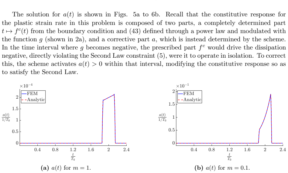
For the quasi-static, rate-dependent elastoplastic bar, the paper's central discovery is that the dissipation inequality $l(f^c+a) = s^2/2 \ge 0$ can be treated as an algebraic constraint in a constrained optimization problem. The pointwise minimizer of $H = \int_0^T (\tfrac12 c_a a^2 + \tfrac12 c_s s^2)\,dt$ subject to this constraint and $p_t = f^c + a$ is $s^2 = 0$ when $f^c < (c_s/c_a)l$ and $s^2 = 2l(f^c - (c_s/c_a)l)$ otherwise, which in the limit $c_s\sigma_0/(c_a\hat\gamma)\to 0$ gives $p_t = \max(f^c,0)$. Thus when the prescribed constitutive response $f^c$ is negative, the correction $a$ cancels it and the plastic strain rate vanishes, keeping dissipation exactly at zero and satisfying the Second Law at every instant. The claimed outcome is a well-set procedure that selects the minimal deviation from the specified constitutive law among the infinite family of solutions satisfying equilibrium, the constitutive equation, and the Second Law.
Load-bearing premise
The argument stands on the premise that minimizing the quadratic cost $H$ selects the physically relevant solution, and the reported numerical match to that minimizer relies on a hand-picked small initial base state $\bar s$, since $\bar s=0$ freezes the dissipation variable at zero and large $\bar s$ converges to different solutions of the same primal system.
Editorial extensions
If this is right
- If a constitutive model violates the Second Law, the scheme repairs it by setting plastic strain rate to zero in the offending interval, producing 'elastic gaps' in the stress-strain response.
- The method provides a practical way to couple established constitutive models for disparate phenomena without first deriving complicated Second Law restrictions on the joint response.
- The computational scheme extends to systems where eliminating differential constraints analytically is not feasible, since it solves the primal equations through a convex dual functional.
- The selected minimal correction depends on the ratio $c_s/c_a$; as this ratio goes to zero, the correction becomes the simple rectifier $p_t = \max(f^c,0)$.
- The solution family is infinite, and the minimization chooses one member, while the numerical method's choice is guided by the initial base state.
Reading between the lines
- The base-state dependence suggests the variational problem is not fully self-contained as a selection criterion: the analytical minimizer (10)-(11) is recovered numerically only because a small nonzero $\bar s$ is hand-chosen, so a principled selection rule would require an additional physical criterion or a limit procedure.
- The same machinery could be used to correct other constitutive inequalities, such as entropy production constraints in heat or mass transport, by replacing the inequality with a minimal additive control field.
- A testable extension is to replace the quadratic cost by an $\ell^1$ cost on $a$, which would yield a sparse correction active only where needed; comparing predictions in the transition regions could discriminate the cost choice.
- The infinite family of solutions parametrized by the dissipation function shows that the Second Law alone does not pin down plastic response; the physical content is carried by the choice of cost functional.
Editorial analysis
A structured set of objections, weighed in public.
Referee Report
Summary. This paper proposes a variational procedure for enforcing the Second Law when the constitutive specification for the plastic strain rate is faulty. For a one-dimensional rate-dependent elastoplastic bar under a prescribed force, the authors assume p_t = f^c(l(t),t) + a(x,t), impose equilibrium and the dissipation inequality l(f^c+a) - s^2/2 = 0, and minimize the quadratic objective ∫(1/2 c_a a^2 + 1/2 c_s s^2)dt subject to those constraints. The closed-form pointwise minimizer is derived in Eq. (12), and in the limit c_s σ_0/(c_a γ̂) → 0 it reduces to p_t = max(f^c,0), so that the dissipation inequality holds even when the prescribed f^c is negative. The paper then develops a dual variational, DtP-based computational scheme following earlier work by the same group, and reports good agreement with the analytic solution for two material exponents. Crucially, the paper also states that the numerical scheme minimizes a sequence of functionals H_k with changing base states rather than the original H, and that the agreement is due to the small initial base state s̄, which acts as a selection parameter among infinitely many solutions of the primal system.
Significance. If the computational branch were justified, this paper would provide a concrete, checkable demonstration that a faulty constitutive specification can be corrected by the minimal additive control enforcing non-negative dissipation, which is a genuinely useful idea for complex constitutive modeling. The closed-form section is transparent and the derivation of Eq. (12) is straightforward to verify; the limiting result p_t = max(f^c,0) is clean and central. However, the numerical validation currently reduces to showing that a small initial base state selects the analytic branch of an infinite solution family. No principled criterion for that selection is provided, and the paper candidly admits that other base states converge to different solutions that also satisfy equilibrium, the constitutive equation, and the Second Law. The abstract and conclusion claim the computational solutions are 'accurate' and provide 'numerical confirmation', but that claim is not established for the stated minimization problem (10)-(11).
major comments (3)
- [Sec. 3.1, Eq. (18), Table 2] The numerical equivalence claim is not established for the stated problem (10)-(11). The DtP map (18) gives s_H = c_s s̄/(α+c_s), which is homogeneous in s̄; setting s̄ = 0 traps s_H = 0 for the entire computation. The authors initialize s̄ = 0.1 and explicitly state in Sec. 3.1 that the initial base state acts as a selection parameter and that values of order 1e6 converge to a different solution of the primal system. Since no criterion is given for choosing the base state, and no proof connects the base-state sequence to the minimizer of H, the reported errors below 0.8% are properties of the hand-picked initialization rather than of the minimization problem the paper claims to solve.
- [Sec. 3.1, paragraph after Eq. (45)] The manuscript itself concedes that 'strictly speaking, the numerical scheme does not attempt to discretize the problem defined by (10)-(11)' and that it works instead with a sequence of functionals H_k parametrized by changing base states. This is a load-bearing limitation, not a minor caveat: the abstract and conclusion credit the accuracy of the computational scheme to the dual variational formulation, but the formulation as implemented is a different algorithm. The paper needs either a convergence argument showing that the fixed point of the base-state update minimizes the original H, or a recharacterization of the numerical results as a sensitivity study of the base-state selection.
- [Sec. 4, Conclusion] The conclusion that the results 'provide a first numerical confirmation that the dual variational principle ... is capable of enforcing the Second Law' is stronger than the evidence supports. Given the paper's own acknowledgment that the initial s̄ is a free selection parameter and that different s̄ values yield different valid solutions, the numerical experiments confirm only that one particular selection reproduces the analytic branch. The claim of numerical confirmation should be either withdrawn or accompanied by a well-defined selection rule (for example, a continuation argument from the exactly solved limit, or a proof of Γ-convergence of the H_k sequence).
minor comments (6)
- [Sec. 2, Eq. (12)] The assumption in Sec. 2 is stated as l(t) ≥ 0, but the constraint (11a) divides by l(t); the closed-form formula (12) should be stated for l(t) > 0, with the initial instant l(0)=0 treated as a limit.
- [Fig. 9b caption] The caption for Fig. 9b says 'Dissipated energy for m=1 case', but the figure and surrounding text describe the m=0.1 case; this appears to be a typo.
- [Eq. (45)] The notation m(v_r(t)) is described as 'the mean of v_r(t) in the physical time domain', but the formula is unclear about whether this mean is over all time or a local average; please define it precisely.
- [Table 1] The algorithm text contains a typographical error: 'F or n≥0' should read 'For n≥0'.
- [Sec. 3, Eq. (16) and surrounding text] The notation D is used both for the ordered pair (D, D_t) and for the dual field itself; this is confusing and should be disambiguated, for instance by writing D = (α, β) and D_t = (α_t, β_t).
- [Sec. 3, Eq. (15) vs Eq. (10)] The same symbol H is used for the physical objective in Eq. (10) and for the auxiliary potential in Eq. (15); although the text explains the relation, different symbols (e.g., H_phys and H_aux) would greatly improve readability.
Circularity Check
Closed-form derivation is self-contained; computational accuracy claims are steered by the base-state selection parameter, making the numerical validation partially circular.
-
fitted input called prediction
[Sec. 3.1 (Results), final paragraph; cf. Eq. (18) DtP map s_H = c_s ¯s/(α+c_s)]
"Numerical experiments (not shown) with initial values of ¯s of the order of 1×10^6 converge to a different solution of the primal system, still satisfying force equilibrium, the constitutive equation, and the Second Law, but does not resemble the analytical solution obtained by minimizing H. This confirms that the initial value of the base state is acting as a selection parameter among infinite possible solutions, and that the small value of ¯s used here guides the scheme toward the desired closed-form solution, within the errors reported above."
The DtP map (18) gives s_H = c_s ¯s/(α+c_s), so the base state ¯s linearly selects the s-branch that the iterative scheme can explore: ¯s = 0 traps s_H = 0, while large ¯s converges to a different member of the infinite family of primal solutions that also satisfy equilibrium, the constitutive relation, and the Second Law. The paper chooses ¯s = 0.1 precisely to remain close to the closed-form minimizer, and then reports agreement with that minimizer. Thus the reported sub-0.8% errors are not an independent confirmation that the algorithm solves the minimization problem (10)-(11); they are a consequence of the hand-picked selection parameter.
full rationale
The analytic solution of Sec. 2 is derived directly from the objective (10) and constraints (11), with no circular dependence on the cited dual variational framework; the limit giving p_t = max(f^c, 0) follows algebraically from (12). The numerical section imports its dual variational machinery and convergence strategy from the authors' own prior work ([1], [3], [11]), but those citations are not the source of the closed-form result. The genuine circularity is in the computational validation: the algorithm's output branch is selected by the initial base state, as the paper itself acknowledges. Since ¯s = 0 traps s_H = 0 and larger ¯s selects other valid solutions, the choice ¯s = 0.1 effectively uses knowledge of the desired analytical solution to guide the scheme toward it. Consequently, the reported accuracy of the computational method is a property of the initialization, not an independent demonstration that the stated minimization problem (10)-(11) is solved. This is a partial circularity of the numerical prediction, while the central analytical derivation remains self-contained.
Assumptions & free parameters
free parameters (4)
- c_a =
1e15 sigma_0 T_0^2
- c_s =
1e3 T_0
- c_p =
1e3 sigma_0
- initial base states (bar-p, bar-s, bar-a) =
0, 0.1, 0
assumptions (5)
- domain assumption Dissipation inequality in the isothermal 1D setting takes the form sigma p_t >= 0 (Eq. 5)
- domain assumption Additive decomposition of strain and quadratic free energy (Eq. 4)
- ad hoc to paper Plastic strain rate has the form p_t = f^c(sigma,t) + a(x,t) (Eq. 8)
- domain assumption x-independent fields suffice for the 1D problem (Sec. 2, 'ansatz we adopt')
- domain assumption Convexity and convergence of the dual functional rely on theorems from refs. [3] and [11]
invented entities (1)
-
a(x,t): additive correction to the prescribed plastic strain rate
Cite this review
Pith. "Pith review of Solving the Dissipation Inequality not as a constitutive restriction." pith.science (2026). https://pith.science/paper/QASQWEJ2
@misc{pith2026260802215,
  author       = {Pith},
  title        = {Pith review of: Solving the Dissipation Inequality not as a constitutive restriction},
  year         = {2026},
  howpublished = {\url{https://pith.science/paper/QASQWEJ2}},
  note         = {Machine review of arXiv:2608.02215}
}
read the original abstract
A solution procedure is formulated and solved for treating the nonlinear Dissipation Inequality as a constraint equation within continuum mechanics, and allowing for incomplete knowledge of constitutive behavior. The scheme is demonstrated in the context of the rate-dependent, elastoplastic response of a bar, resulting in a nonlinear problem of constrained optimization. Both closed form and computational results are developed. The computational solutions utilize a sequence of convex optimization problems, and are shown to be accurate. In the example considered, the approach is shown to automatically correct an (intentionally) faulty constitutive specification, resulting in the solution to be in accord with the fundamental postulates of continuum mechanics.
Figures


Figures from the paper (16 more)




Reference graph
Works this paper leans on
-
[1]
Mechanics Research Communications , volume=
The Second Law as a constraint and admitting the approximate nature of constitutive assumptions , author=. Mechanics Research Communications , volume=. 2025 , publisher=
work page 2025
-
[2]
Fleck, N. A. and Hutchinson, J.W. and Willis, J.R. , pages=. Guidelines for constructing strain gradient plasticity theories , journal=. 2025 , publisher=
work page 2025
-
[3]
European Journal of Mechanics-A/Solids , volume=
Discrete defect plasticity and implications for dissipation , author=. European Journal of Mechanics-A/Solids , volume=. 2023 , publisher=
work page 2023
-
[4]
Hidden convexity in the heat, linear transport, and
Kouskiya, Uditnarayan and Acharya, Amit , journal =. Hidden convexity in the heat, linear transport, and
-
[5]
Acharya, Amit , journal=. A new perspective in linear. 2026 , url=
work page 2026
-
[6]
Journal of Elasticity , volume=
A dual variational principle for nonlinear dislocation dynamics , author=. Journal of Elasticity , volume=. 2023 , publisher=
work page 2023
-
[7]
Variational principles for nonlinear
Acharya, Amit , journal=. Variational principles for nonlinear
- [8]
Show all 19 references
-
[9]
, TITLE =
Acharya, Amit and Sengupta, Ambar N. , TITLE =. Proc. of the Royal Society A. , FJOURNAL =. 2024 , NUMBER =
2024
-
[10]
Variational formulation based on duality to solve partial differential equations: Use of
Sukumar, N and Acharya, Amit , journal=. Variational formulation based on duality to solve partial differential equations: Use of. 2025 , publisher=
2025
-
[11]
Mathematics and Mechanics of Solids , year =
A hidden convexity in continuum mechanics, with application to classical, continuous-time, rate-(in)dependent plasticity , author =. Mathematics and Mechanics of Solids , year =
-
[12]
On the variational dual formulation of the
Vorotnikov, Dmitry and Acharya, Amit , journal=. On the variational dual formulation of the
-
[13]
Variational Principle for a Damped, Quadratically Interacting Particle Chain with Nonconservative Forcing
Acharya, Amit and Sengupta, Ambar N. Variational Principle for a Damped, Quadratically Interacting Particle Chain with Nonconservative Forcing. Continuum Models and Discrete Systems. 2024
2024
-
[14]
arXiv e-prints , keywords =
Variational Dual Solutions for Incompressible Fluids. arXiv e-prints , keywords =
-
[15]
arXiv e-prints , keywords =
Variational Dual Solutions of Chern-Simons Theory. arXiv e-prints , keywords =
-
[16]
Journal of Elasticity , volume=
A hidden convexity of nonlinear elasticity , author=. Journal of Elasticity , volume=. 2024 , publisher=
2024
-
[17]
Quarterly of Applied Mathematics , volume =
Kouskiya, Uditnarayan and Acharya, Amit , title =. Quarterly of Applied Mathematics , volume =
-
[18]
and Acharya, Amit , journal=
Kouskiya, Uditnarayan and Pego, Robert L. and Acharya, Amit , journal=. Traveling wave profiles for a semi-discrete. 2025 , url=
2025
-
[19]
arXiv e-prints , year = 2025, url=
A convex variational principle for the necessary conditions of classical optimal control. arXiv e-prints , year = 2025, url=
2025
Reviewed August 10, 2026 · model on record in the stance chip above.
Discussion (0). Continue with ORCID to comment.