REVIEW 4 major objections 5 minor 14 references
This paper makes Markov-chain samplers learn when to stop, proving that unbiased stopping policies for a fixed kernel are characterized by a Poisson equation, and showing that learned stopping cuts trajectory lengths by orders of magnitude
Reviewed by Pith at T0; open to challenge. T0 means a machine referee read the full paper against a public rubric. the ladder, T0–T4 →
T0 review · deepseek-v4-flash
2026-08-02 11:12 UTC pith:32VOT5G6
load-bearing objection Genuine extension of non-acyclic GFlowNets to learned stopping, but the central theorem rests on an unverified ergodicity assumption and the classifier-only ablation undercuts the headline claim; still worth a serious referee. the 4 major comments →
Stop the Sampler! Classifier-Based Adaptive Stopping for Sampling Kernels
The pith
A machine-rendered reading of the paper's core claim, the machinery that carries it, and where it could break.
Core claim
The paper's central claim is that a Markov chain sampler with a learnable stopping probability can be unbiased only if its flow measure solves a Poisson equation determined by the forward kernel. Theorem 3.6 states: for a uniformly geometrically ergodic forward kernel Q_F, detailed balance holds if and only if the flow density has the form f = Z(u + n_Q π_Q), the forward stopping classifier is d_F = r/f, and the minimal admissible n_Q gives exactly the minimal mean trajectory length. This establishes a constructive link between optimal stopping classifiers and the target density: the classifier behaves like the ratio of target to flow, returning higher stopping probabilities in high-density
What carries the argument
The central objects are the flow measure F, defined as the expected number of visits to each state under the forward kernel, and the two stopping classifiers d_F and d_B that parameterize the stopping decision. Detailed balance forces d_F = r/f and d_B = Z p0/f, and Theorem 3.6 turns these into the Poisson equation (I - Q_F)V = p0 - π_Q for the normalized flow V = F/Z. Solving this equation yields both the classifier and the minimal mean trajectory length n*_Q; the training objective is a prefix trajectory balance loss with flow regularization.
Load-bearing premise
The main theorem assumes the fixed forward kernel Q_F is uniformly geometrically ergodic with a unique stationary measure π_Q; if the ULA kernels used in the experiments do not satisfy this, the characterization of admissible stopping classifiers and the exact lower bound on trajectory length are not established.
What would settle it
On a low-dimensional target where the Poisson equation can be solved numerically (e.g., a Gaussian with ULA), train the model and check whether the learned classifier satisfies d_F = r/f with f = Z(u + n_Q π_Q) and whether the empirical mean trajectory length attains n*_Q; a substantial deviation would falsify the claim that the learned stopping rule is the unbiased one characterized by Theorem 3.6.
If this is right
- For any fixed forward kernel Q_F, unbiased sampling with learned stopping requires at least n*_Q steps on average; the classifier must satisfy d_F = π/(u + n_Q π_Q), so the theory pins down both the shortest feasible trajectory and the stopping rule that achieves it.
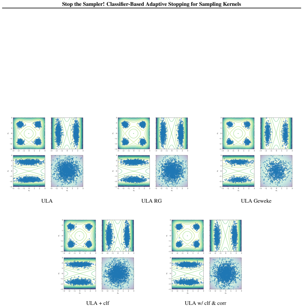
- A learnable correction to the forward kernel lets the sampler jump between modes, overcoming the slow mixing that plain ULA exhibits on multimodal targets like GMM9 and ManyWell.
- The learned classifier visually recovers the target geometry, assigning higher stopping probability in high-density regions, which gives an interpretable signal of where the sampler considers its job done.
- The multilevel variant with annealed intermediate rewards extends the same framework to high-dimensional tasks (e.g., d=196), where it becomes competitive with dedicated diffusion-based samplers while using comparable or fewer steps.
Where Pith is reading between the lines
- We infer that the framework interpolates between MCMC and amortized generative sampling: when the learned mean trajectory length n_Q runs near its lower bound n*_Q, the method behaves like a flow-based sampler, while larger n_Q recovers standard MCMC; this suggests a tunable trade-off between compute budget and statistical efficiency that practitioners could dial in per application.
- A direct test of the theory would be to solve the Poisson equation (63) numerically on a simple target (e.g., a Gaussian with a ULA kernel), compute n*_Q and d_F = r/f, and compare the trained classifier and empirical mean trajectory length against those values; mismatch would indicate either optimization failure or that the uniform-geometric-ergodicity assumption does not hold.
- If uniform geometric ergodicity fails for heavy-tailed targets such as the Funnel, the theorem's formulas may still serve as a heuristic — the classifier should approximate r/f — but the unbiasedness guarantee and the exact lower bound would need a generalization of potential theory beyond uniform ergodicity (e.g., using a solution of the Poisson equation in a weaker sense).
Editorial analysis
A structured set of objections, weighed in public.
Referee Report
Summary. The paper proposes to treat trajectory termination in continuous sampling as a learnable component, framed as a non-acyclic GFlowNet. The state space is R^d plus source and sink states; forward/backward policies include state-dependent stopping classifiers d_F and d_B, and training uses a prefix trajectory-balance objective with flow regularization. A multilevel extension interpolates between an initial distribution and the target by a sequence of annealed rewards. The main theoretical result, Theorem 3.6, characterizes all detailed-balance solutions for a fixed uniformly geometrically ergodic kernel Q_F: the flow must be of the form Z(U + n_Q π_Q), the classifiers satisfy d_F = r/f and d_B = Z p0/f, and the mean trajectory length equals n_Q. Experiments compare ULA, ULA with learned stopping, ULA with learned stopping and drift correction, and multilevel samplers on several targets, and report reduced trajectory lengths and competitive or improved sample metrics relative to ULA and some diffusion-sampler baselines.
Significance. The framework is interesting: it gives a clean expected-trajectory identity (Prop. 3.5), connects non-acyclic GFlowNets to MCMC-style stopping, and the authors provide code. The multilevel extension is a reasonable practical contribution. If Theorem 3.6 were established under checkable assumptions, the characterization of admissible classifiers and flow measures would be a useful theoretical bridge. However, as it stands the central theorem rests on a strong uniform ergodicity assumption that is not verified for any kernel used in the experiments, and the fixed-kernel classifier-only experiment in Table 1 does not show the unbiasedness the theorem promises. The improved empirical results come from the learned-drift variant, which is outside the theorem's scope. With those gaps addressed, the paper could make a solid contribution; in its current form the central claim is not yet supported.
major comments (4)
- [Section 3.2, Theorem 3.6 and Eq. (17)] The central theorem assumes the fixed kernel Q_F is uniformly geometrically ergodic with stationary measure π_Q. This is not verified for the ULA kernels used in Table 1 (GMM9, Funnel, ManyWell) or for the Digits NICE-flow target in Table 2. Uniform geometric ergodicity of fixed-step ULA is not guaranteed for heavy-tailed targets such as Funnel, and no drift/minorization check is supplied. If Eq. (17) fails, the series defining U in Eq. (19) need not converge, the Poisson equation (63) need not have the claimed solution class, and the formulas d_F=r/f, d_B=Zp0/f and q_B in Eq. (20) are unsupported. Since Theorem 3.6 is the theoretical basis for the claim that a learned classifier can de-bias a fixed MCMC kernel, this is a load-bearing issue. Please verify the condition for the actual kernels, restrict the claim to kernels for which it is known to hold, or provide a sensitivity analysis s
- [Table 1, GMM9 (d=2) row] The row 'ULA w/ clf' is exactly the fixed-q_F setting of Theorem 3.6: q_F is the ULA kernel and only d_F, d_B, q_B are learned. Compared with ULA, the learned sampler reduces mean trajectory length from 10^4 to 15, but SD worsens from 0.463 to 1.522 and MMD worsens from 0.002 to 0.053. If Theorem 3.6 applied and training converged to a detailed-balance solution, terminal samples would be unbiased; the observed degradation indicates either the theorem's assumptions fail or the prefix-TB objective (22) does not converge to such a solution. The paper does not report TB/DB residuals or n_Q^* from Cor. 3.7, so the reader cannot tell which. Meanwhile the improved metrics in Table 1 come from 'ULA w/ clf & corr', where q_F is learned and therefore outside the scope of Theorem 3.6. This gap must be resolved before the headline claim is supported.
- [Appendix D.4, Eqs. (63), (65) and Eq. (19)] The detailed-balance derivation yields V(I-Q_F) = p0 - π Q_F, where π is the target density. The proof and theorem state the series for U using the symbol π_Q^{n+1}_F. If this denotes π_Q Q_F^{n+1} = π_Q for the stationary measure, the telescoping gives p0 - π_Q, not p0 - π Q_F, and the characterization would only hold when π = π_Q. If it denotes π Q_F^{n+1} with the target π, the notation collides with the stationary measure π_Q and the equations are not readable as printed. Please rewrite the series and the Poisson equation with explicit measures and re-verify the derivation.
- [Cor. 3.7 and Eq. (19), n_Q^*] The theorem requires the supremum n_Q^* to be finite, and Cor. 3.7 identifies n_Q with the mean trajectory length. The paper never checks finiteness of n_Q^* or the positivity/well-definedness of the denominator π_Q(s). For ULA on heavy-tailed targets, π_Q is Gaussian-like while the target π can have much heavier tails, so (max{π,p0}-u)/π_Q may be unbounded; even in lighter-tailed cases π_Q(s) may be arbitrarily small. Additional assumptions or numerical checks are needed for the theorem and corollary to apply to the experimental settings.
minor comments (5)
- [Section 2.1] There is a leftover LaTeX command '§gobble 3.1' in the text; please fix.
- [Acknowledgments] 'Acknowledgmenents' is a typo for 'Acknowledgements'.
- [Section 3.4, Prop. 3.8] Proposition 3.8 is called 'evident' but is the correctness argument for the multilevel sampler. Please provide a proof or a reference; the claim is not merely presentational.
- [Eq. (22) and Algorithm 1] The stop-gradient notation 'sg' is introduced only in Eq. (22), and the trajectory notation 'eτ' and 'τ^b_{0:i}' in Algorithm 1 is not defined. Please clarify these before use.
- [Table 1] The baseline expected trajectory lengths are formatted inconsistently (e.g., '10 4', '5×10 2', '1.5×10 3'). Please make the table entries unambiguous.
Circularity Check
No significant circularity: core derivation is in-paper; self-citations are non-load-bearing technical foundations.
full rationale
The central theoretical claim (Thm 3.6) is derived in Appendix D.4 from the detailed balance equations themselves: the Poisson equation (63) follows from integrating the interior DB condition, and the solution family U + n_Q pi_Q is obtained by solving that equation under uniform geometric ergodicity (17). The classifier identities d_F = r/f and d_B = Zp0/f are literally the DB equations at the sink and source (59), not a fitted relation renamed as a prediction. The target r appears as the problem reward, which is the input of a sampling algorithm, so its use in training is not circular. The identity E[n_tau] = F(S)/F({s0}) (Prop. 3.5) follows immediately from the explicit occupancy definition of F (Def. 3.2); the paper transparently turns this identity into the flow regularizer rho r(s_i)/d_F(s_i) exactly because r/d_F = f, so the reported short trajectories are an engineered objective, not an independent prediction. The unverified uniform ergodicity of ULA kernels (Eq. 17) is a correctness/robustness concern, not a circularity: the theorem's conclusion is conditional on that assumption. Self-citations (Morozov et al. 2025, 2026; Gritsaev et al. 2025) supply technical components (prefix TB, flow regularization), but the paper states the objectives explicitly and the core equivalence is proved in-paper, so they are non-load-bearing. No step reduces by construction to its own input. Score 2 reflects only minor non-load-bearing self-citation, not substantive circularity.
Axiom & Free-Parameter Ledger
free parameters (5)
- flow regularization coefficient ρ =
0.1 (GMM9 d=2, ManyWell d=40), 1.0 (GMM9 d=40, Digits), 0.01 (Funnel)
- Langevin step size γ =
0.1 or 0.01 per environment
- maximum training trajectory length N_max =
100 (most), 50 (Digits)
- classifier lower bound ε =
1e-5
- initial variance σ0² =
1 (low-dimensional), 5 (high-dimensional)
axioms (4)
- domain assumption GFlowNet flow-matching and reward-matching theorems from Lahlou et al. (2023) apply in the non-acyclic continuous setting.
- domain assumption Assumption 3.1: the trajectory distribution induced by the forward kernel has finite expected length.
- domain assumption The fixed forward kernel Q_F is uniformly geometrically ergodic with unique stationary measure π_Q (Eq. 17).
- domain assumption The target reward r is known pointwise and its gradient is available.
read the original abstract
Sampling from complex, unnormalized probability densities is a fundamental challenge in Bayesian inference and probabilistic modeling. While Markov chain Monte Carlo (MCMC) methods provide asymptotic guarantees, they often suffer from slow mixing and high computational costs due to fixed or manually tuned trajectory lengths. In this work, we propose a novel framework that treats trajectory termination as a learnable component of the sampling dynamics. By framing MCMC within the theory of non-acyclic generative flow networks (GFlowNets), we train state-dependent neural classifiers to decide when a trajectory has reached a high-density region and should terminate. We theoretically establish the connection between optimal classifiers and the target density via detailed balance conditions and introduce a multilevel training scheme to facilitate exploration in complex geometries. Experimental results across various benchmark densities demonstrate that our approach significantly reduces average trajectory lengths while improving mode coverage and mixing compared to standard MCMC baselines.
Figures



Reference graph
Works this paper leans on
-
[1]
At each iteration, the algorithm alternates between forward (on-policy) and backward (off-policy) updates
In this section, we provide additional implementation details. At each iteration, the algorithm alternates between forward (on-policy) and backward (off-policy) updates. During forward updates, trajectories are sampled from the forward policy starting from the initial distribution 𝑝0. During backward updates, terminal states are sampled from a replay buff...
2024
-
[2]
Environment↓Parameter→lr𝜌 𝛾 𝑁 max grad clip GMM9 (𝑑=40)10 −4 100 10−1 102 10−3 ManyWell (𝑑=40)10 −5 10−1 10−2 102 10−5 Digits (𝑑=196)10 −4 100 10−1 5×10 1 10−3 A.6
Table 4.Environment-specific hyperparameters for multi-level experiments, where lr is a learning rate of the optimizer,𝜌 is a regularization coefficient,𝛾 is the step-size,𝑁max is trajectory length during training and grad clip specifies values of the gradient clipping with respect to parameters in the optimizer. Environment↓Parameter→lr𝜌 𝛾 𝑁 max grad cli...
2024
-
[5]
Wang, C., Chen, W., Kanagawa, H., and Oates, C. J. Rein- forcement learning for adaptive MCMC.Artificial Intelli- gence and Statistics (AISTATS), 2025a. Wang, C., Fisher, M. A., Kanagawa, H., Chen, W., and Oates, C. J. Harnessing the power of reinforce- ment learning for adaptive MCMC.arXiv preprint arXiv:2507.00671, 2025b. Welling, M. and Teh, Y . W. Bay...
-
[12]
LetH𝑘 be the RKHS associated with a positive definite kernel𝑘
is a kernel-based integral probability metric that compares two distributions through their embeddings in a reproducing kernel Hilbert space (RKHS). LetH𝑘 be the RKHS associated with a positive definite kernel𝑘. The MMD between𝑝 𝑇 and𝜋is defined as MMD𝑘(𝑝𝑇,𝜋)=sup 𝑓∈H 𝑘 ∥𝑓∥ H𝑘≤1 E𝑥∼𝑝𝑇[𝑓(𝑥)]−E 𝑦∼𝜋[𝑓(𝑦)] .(27) For characteristic kernels, this quantity is non...
2024
-
[13]
based on the quadratic cost. The underlying unregularized quantity is the 2-Wasserstein distance, 𝑊2,𝜀(𝑝𝑇,𝜋)=inf 𝜉∈Γ(𝑝 𝑇,𝜋) ∫ R𝑑×R𝑑 ∥𝑥−𝑦∥ 2 2𝜉(𝑑𝑥,𝑑𝑦)−𝜖H(𝜉) 1/2 ,(30) whereΓ(𝑝𝑇,𝜋) denotes the set of couplings with marginals 𝑝𝑇 and𝜋, andH(𝜉)=− ∫ R𝑑×R𝑑𝜉(𝑥,𝑦)log𝜉(𝑥,𝑦)d𝑥d𝑦 . In practice, we compute its entropically regularized counterpart using Sinkhorn iterat...
2024
-
[14]
was introduced, but it requires samples from𝜋: log𝑍=E 𝑥∼𝜋,𝜏∼𝑝 𝐵(·|𝑠𝑛𝜏=𝑥) log𝑟(𝑥)𝑝 𝐵(𝜏|𝑠 𝑛𝜏 =𝑥) 𝑝𝐹(𝜏) −KL(𝜋·𝑝 𝐵||𝑝 𝐹)≤E 𝑥∼𝜋,𝜏∼𝑝 𝐵(·|𝑥) log𝑟(𝑥)𝑝 𝐵(𝜏|𝑠 𝑛𝜏 =𝑥) 𝑝𝐹(𝜏) . (34) We draw𝑀=2000samples from𝜋and then simulate trajectories using a backward policy: EUBO= 1 𝑀 𝑀∑︁ 𝑖=1 log𝑟(𝑥 𝑖)+log𝑝 𝐵(𝜏𝑖|𝑠 𝑛𝜏 =𝑥 𝑖)−log𝑝 𝐹(𝜏𝑖) , 𝑥 𝑖∼𝜋,𝜏 𝑖∼𝑝 𝐵(·|𝑠 𝑛𝜏 =𝑥 𝑖).(35) A.7. Additio...
2024
-
[128]
The forward continuous kernel𝑞𝐹 is either fixed (in the ULA-based setup) or augmented with learned drift and variance corrections, while the backward kernel is always learned. The forward and 12 Stop the Sampler! Classifier-Based Adaptive Stopping for Sampling Kernels Algorithm 1Training non-acyclic continuous GFlowNet with prefix trajectory balance Input...
2000
-
[2011]
Wu, J. and Kawai, R. Stopping rules for Monte Carlo methods: A review.arXiv preprint arXiv:2510.22688,
-
[2012]
Adaptive destruction processes for diffusion samplers
Gritsaev, T., Morozov, N., Tamogashev, K., Tiapkin, D., Samsonov, S., Naumov, A., Vetrov, D., and Malkin, N. Adaptive destruction processes for diffusion samplers. arXiv preprint arXiv:2506.01541,
-
[2022]
Experimental details A.1
10 Stop the Sampler! Classifier-Based Adaptive Stopping for Sampling Kernels A. Experimental details A.1. Continuous kernels parameterizations We initialize trajectories from the Gaussian distribution 𝑝0(𝑠)=N(𝑠|0,𝜎 2 0𝐼). For transitions between continuous states, we use the forward density 𝑞𝐹(𝑠′|𝑠;𝜃)=N (𝑠′|𝜇𝐹(𝑠;𝜃),Σ 𝐹(𝑠;𝜃)), 𝜇𝐹(𝑠;𝜃)=𝑠+𝛾 𝑢𝐹(𝑠;𝜃)+ 1+𝑣 𝐹(𝑠;...
2022
-
[2023]
NICE: Non-linear independent components estimation.arXiv preprint arXiv:1410.8516,
Dinh, L., Krueger, D., and Bengio, Y . NICE: Non-linear independent components estimation.arXiv preprint arXiv:1410.8516,
-
[2024]
The target distribution is a continuous density over R196, obtained by training an invertible flow on 14×14 MNIST images
and corresponds to sampling MNIST images from a density defined by a NICE normalizing flow model (Dinh et al., 2014). The target distribution is a continuous density over R196, obtained by training an invertible flow on 14×14 MNIST images. Although the underlying dataset consists of images, the resulting target distribution has full support on R196. Sampl...
2014
-
[2025]
Learning shortest paths with generative flow networks
Morozov, N., Maksimov, I., Tiapkin, D., and Samsonov, S. Learning shortest paths with generative flow networks. arXiv preprint arXiv:2603.01786,
-
[2026]
Deleu, T. and Bengio, Y . Generative flow net- works: a markov chain perspective.arXiv preprint arXiv:2307.01422,
discussion (0)
Sign in with ORCID, Apple, or X to comment. Anyone can read and Pith papers without signing in.