REVIEW 3 major objections 3 minor 40 references
This paper establishes that the statistical value of depth in message passing on a sparse graph is governed by a single Kesten–Stigum ratio κ=γ²Δ, with error saturating geometrically below κ=1 and compounding geometrically above it.
Reviewed by Pith at T0; open to challenge. T0 means a machine referee read the full paper against a public rubric. the ladder, T0–T4 →
T0 review · deepseek-v4-flash
2026-08-01 20:16 UTC pith:4XPD3GXQ
load-bearing objection A careful theory paper that proves a clean Kesten-Stigum dichotomy for the value of depth in sparse-CSBM message passing, but the below-threshold half rests on a symmetry assumption the paper concedes is open when relaxed. the 3 major comments →
The Value of Depth in Message Passing on Sparse Graphs: A Kesten-Stigum Dichotomy
The pith
A machine-rendered reading of the paper's core claim, the machinery that carries it, and where it could break.
Core claim
On the limit tree, the classifier aggregates distance-attenuated evidence 2 artanh(γ^k t(X_v)) from every vertex at distance k. The paper's central discovery is that the entire error map E(ℓ) is governed by κ=γ²Δ. The key mechanism is an antisymmetry identity: under symmetric feature classes, the expected message from generation k is exactly opposite for the two labels, so generation-k evidence scales as κ^k rather than the naive (γΔ)^k, and its second moment vanishes geometrically when κ<1. This yields a geometric saturation theorem below the threshold (Theorem 3.1), a matching κ^{ℓ/2} decision-flip lower bound (Theorem 3.2), and a geometric amplification theorem above it (Theorem 3.3). A u
What carries the argument
The central object is the Kesten–Stigum ratio κ=γ²Δ, the square of the edge signal times the average degree, which is the same quantity that separates reconstructible from non-reconstructible broadcast processes. It is carried by two identities: the message antisymmetry E_−[M_k] = −E_+[M_k] for the clipped feature messages M_k(x) = 2 artanh(γ^k t(x)), and the broadcast/branching martingale W_k = D_k/(γΔ)^k, whose L² behavior is summable exactly when κ<1. Together they show that the net evidence of generation k has mean of order κ^k and fluctuation of order κ^{k/2}, so κ acts as the per-layer signal-to-noise gain; the same ratio reappears in the first layer's information budget.
Load-bearing premise
The below-threshold saturation proof relies on Assumption 1, that the two feature classes are symmetric via a measure-preserving involution (the Gaussian mixture with opposite means being the canonical case); without this symmetry, generation-k messages acquire a label-independent drift that the sign statistic does not re-center, and the stated κ^{ℓ/3} saturation may fail.
What would settle it
Simulate the classifier on broadcast-labeled Poisson Galton–Watson trees with asymmetric feature classes (e.g., N(µ,σ²) under label +1 and N(−µ,2σ²) under label −1) at κ<1 and measure |E(ℓ)−E(ℓ+1)|; if it does not decay geometrically at a rate governed by κ (or at least at the Lévy-form rate the appendix gives), the symmetry assumption is load-bearing.
If this is right
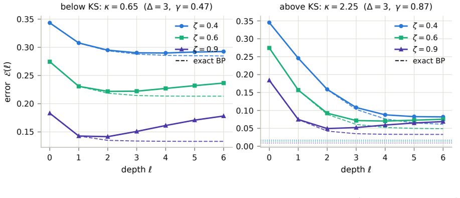
- Below the threshold (κ<1), all layers beyond O(log(1/ε)) combined change the error by less than ε, so on sparse graphs statistical gains from extra depth are exhausted at a bounded, size-independent horizon.
- Above the threshold (κ>1), each additional layer multiplicatively improves the decision statistic, approaching a floor set by branching-process fluctuations that no amount of depth can repair.
- No local classifier of any depth can beat the isolated-root floor e^{-Δ}Φ(−ζ), so depth is never a substitute for feature quality on sparse graphs.
- The first layer strictly improves on feature-only classification by an explicit amount, so even where deep layers saturate, shallow message passing is provably useful.
- Because the pairwise rule treats correlated deep evidence as independent, its error curve has a finite optimal depth; depth should be tuned as a hyperparameter rather than increased monotonically.
Where Pith is reading between the lines
- If this dichotomy transfers to trained GNNs, it predicts an information-limited regime in sparse graphs where depth should scale with log(1/ε), not with graph size or diameter—a testable design rule beyond the pairwise rule analyzed here.
- For asymmetric or unbalanced feature classes, the exact cancellation that powers the below-threshold theorem fails; a natural extension is to test whether a recentred statistic restores geometric saturation, a case the paper leaves open.
- The exact-BP baseline suggests that belief propagation saturates at a strictly faster per-layer ratio κ_BP < κ; proving this would require controlling the stationary law of the nonlinear BP message recursion, which the paper identifies but does not establish.
- For multi-class models, the natural conjecture is to replace γ by the second eigenvalue λ of the class-transition matrix and use κ=λ²Δ as the organizing threshold, following the extension logic the paper sketches.
Editorial analysis
A structured set of objections, weighed in public.
Referee Report
Summary. The paper analyzes the depth-error tradeoff of the pairwise message-passing classifier h_ℓ = sgn(T_ℓ) on the local weak limit of the sparse CSBM, a broadcast-labeled Poisson Galton-Watson tree. The central claim is a Kesten-Stigum dichotomy organized by κ = γ²Δ. Below threshold (κ<1), Theorem 3.1 gives a geometric Cauchy bound on the error sequence, with Theorem 3.2 providing a matching κ^{ℓ/2} lower bound on decision flips; above threshold (κ>1), Theorem 3.3 bounds the error by a branching-process floor plus super-geometric signal terms. The paper also proves a universal floor, a certified strict first-layer improvement, finite-depth prescriptions O(log(1/ε)), identifies the pairwise rule as linearized belief propagation, and documents non-monotonicity of the depth-error curve with an exact certified instance. Simulations with an exact BP baseline and finite-graph transfer experiments accompany the theory, and the paper is unusually explicit about what its constants do and do not certify.
Significance. If the main dichotomy holds as stated, this is a valuable quantitative contribution to the theory of GNN depth on sparse graphs: it identifies a single parameter κ that governs whether additional message-passing layers are information-limited or information-productive, and it gives explicit depth prescriptions independent of graph size. The proofs are coherent second-moment/martingale arguments with a parameter-free derivation of the threshold, and the paper ships reproducible code, a certified non-monotonicity instance with strict error accounting, and a table honestly reporting the vacuity of constants at simulated parameters. These are genuine strengths. However, the below-threshold half is proven only under a symmetric-feature assumption whose removal the paper itself leaves open, the above-threshold theorem is non-vacuous only for κ>17, and the claimed L2 convergence of T_ℓ is not justified by the stated assumptions. These gaps need to be addressed before the dichotomy can be accepted at the level claimed in the abstract.
major comments (3)
- [§2.3, Lemma 4.2(i), §6] The below-threshold dichotomy is proved only under Assumption 1. Lemma 4.2(i) supplies the exact antisymmetry E_-[M_k] = -m_k, and every use of the mean part of Lemma 4.4 depends on it. Without Assumption 1, E[R|G] contains a label-independent drift term of order (γΔ)^k; for Δ=3, γ=0.55 one has κ=0.9075<1 but γΔ=1.65, so this drift can destroy the cancellation that produces the κ^{ℓ+1} rate. Section 6 explicitly states that under class asymmetry the mean message acquires a label-independent drift 'that sgn(T_ℓ) does not re-center' and that saturation for a recentered statistic 'is open.' The abstract and Theorem 3.1 nevertheless state the dichotomy without this caveat. The central below-threshold claim should be restricted to the symmetric-feature CSBM throughout, or extended to a recentered statistic.
- [§4.2, Theorem 3.1] The claim that T_ℓ converges in L2 requires E[(log ψ(X_o))^2] < ∞. Assumption 3 only bounds the density of log ψ(X) by B; a bounded density does not imply a finite second moment (e.g., density proportional to 1/(1+x^2)). Lemma 4.4 proves an L2-Cauchy bound only for the non-root part R; T_0 = log ψ(X_o) may have infinite second moment. As stated, 'T_ℓ converges in L2' is not justified. This does not affect the error-tail bound (6), but it does affect the identification of E(∞) as the error of a bona fide infinite-depth L2 statistic. Add a second-moment assumption (satisfied by the Gaussian example) or replace L2 convergence by convergence in probability/a.s.
- [§3.2, Eq. (7)] The above-threshold bound is non-vacuous only for κ>17: the floor term 16/(κ−1) exceeds 1 for κ≤17. Since κ<Δ, this excludes every sparse configuration with Δ≤17, including the simulated κ=2.25, Δ=3. Thus the theorem as stated does not certify 'depth is geometrically productive' in the sparse regime; the abstract's above-threshold sentence is stronger than what is proved. The paper is admirably explicit in Table 1 about this, but the central statement should be qualified, or the floor constant improved by the kind of left-tail control of W_∞ discussed in §6.
minor comments (3)
- [§2.2] The text refers to 'Theorem 4.2' for antisymmetry of the messages, but the statement is Lemma 4.2. Please correct the cross-reference.
- [§4.3, Step 1] In the proof of Theorem 3.3, the line P(W_1 < 3/4) ≤ 16 Var(W_1) = 16 κ^{-1} uses the exact variance κ^{-1}; the displayed text can be misread as the looser 16/(κ−1). Spell out Var(W_1)=κ^{-1} to avoid confusion.
- [§2.3 / Appendix A] Assumption 3 is described as needed only for Theorem 3.1, but Appendix A immediately provides the Lévy-concentration form that is the right statement for atomic feature laws. Consider moving that remark into Section 2.3 so the scope of Assumption 3 is clear from the outset.
Circularity Check
No significant circularity: the κ-dichotomy is a parameter-free derivation from stated assumptions; self-citations are contextual, not load-bearing.
full rationale
The paper's central dichotomy is derived, not fitted. Theorem 3.1's below-threshold rate κ^{(ℓ+1)/3} follows from the second-moment tail bound in Lemma 4.4, whose cancellation uses Assumption 1 (symmetric features) through Lemma 4.2(i), E_-[M_k]=-m_k. This is an explicitly stated model assumption, not an input that already contains the target theorem; Section 6 openly concedes that without it the mean message acquires a drift and the survival of saturation 'is open', which confirms the result's scope rather than concealing a circularity. Theorem 3.3 above threshold is likewise self-contained and is explicitly flagged as non-vacuous only for κ>17, with its geometric term identified as a truncation cost rather than a signal-driven rate. The classifier h_ℓ is imported from the author's prior work [8], but as the object under study, not as evidence for the new claims; the new theorems are proved from Lemmas 4.1–4.5 and standard branching-process facts. The finite-graph transfer in Remark 3.7 cites [8] but is supported by local weak convergence and by the paper's own finite-n simulations (±0.002 agreement), so it is not load-bearing for the limit-tree dichotomy. Empirically computed quantities—fitted flip rates and κ_BP—are explicitly presented as measurements or annealed predictions, not as theorem inputs. No prediction reduces by construction to a fitted parameter, and no load-bearing conclusion rests solely on a self-citation chain. The honest limitation statements in Section 6 and Table 1 are correctness/scope caveats, not circularity.
Axiom & Free-Parameter Ledger
free parameters (3)
- truncation rate s (Theorem 3.3) =
any s ∈ (0,1)
- effective BP ratio κ_BP = Δ E[F'_γ(L)²] =
√κ_BP ≈ 0.424, 0.559, 0.621 at κ = 1/3, 0.653, 0.923 (ζ=0.6); κ_BP = 0.356 at κ = 2.25
- two-point feature law parameter t0 (Appendix C) =
0.95
axioms (7)
- domain assumption Assumption 1: symmetric mutually absolutely continuous feature classes with measure-preserving involution τ, ρ_− = ρ_+∘τ
- domain assumption Assumption 2: ϑ = E+[t(X)²] > 0 (informative features)
- domain assumption Assumption 3: log ψ(X) has density bounded by B under P+ (non-atomic)
- standard math Local weak convergence of the sparse CSBM to a PGW(Δ) broadcast tree (Aldous–Steele / Benjamini–Schramm, cited [3,9,13,29])
- standard math Kesten–Stigum L² martingale convergence for supercritical GW processes (κ>1): Var(W_∞) ≤ 1/(κ−1) (Lemma 4.3(v))
- standard math Berry–Esseen bound for independent bounded non-identically distributed summands (Petrov, Ch. V)
- domain assumption Δ > 1 throughout (Section 2.1)
invented entities (1)
-
κ_BP = Δ E[F'_γ(L)²], the effective per-layer BP ratio
independent evidence
read the original abstract
How deep does a graph neural network need to be on a sparse graph? We study its purest statistical form: node classification on the sparse contextual stochastic block model (CSBM) with average degree $\Delta=O(1)$, whose local weak limit is a broadcast-labelled Poisson Galton-Watson tree. Prior work derived a message-passing classifier $h_\ell$ that aggregates from each vertex at distance $k\le\ell$ the attenuated evidence $2\operatorname{artanh}(\gamma^k t(X_v))$, with $\gamma$ the edge signal and $t$ a bounded likelihood-ratio transform of the feature. We prove that the value of depth is governed by a single number, the Kesten-Stigum ratio $\kappa=\gamma^2\Delta$. Below the threshold ($\kappa<1$), the error sequence is Cauchy at a geometric rate, $|\mathcal{E}(\ell)-\mathcal{E}(\ell')|\le C\kappa^{(\ell+1)/3}$ for all $\ell'>\ell$, so all layers beyond depth $O(\log(1/\epsilon))$ change the error by less than $\epsilon$; conversely, under mild regularity each sufficiently deep layer still flips the decision with probability at least $c\kappa^{\ell/2}$, the empirically sharp exponent. Above the threshold ($\kappa>1$), depth is geometrically productive: $\mathcal{E}(\ell)$ is driven to a branching-process floor of order at most $1/(\kappa-1)$ at any geometric rate $\kappa^{-s\ell}$, $s<1$ (this bound has content only for $\kappa>17$). No local classifier of any depth beats the universal floor $e^{-\Delta}\Phi(-\zeta)$ set by isolated roots ($\zeta$ the feature signal-to-noise ratio), while the first layer provably helps by an explicit total-variation amount. Simulations with an exact belief-propagation baseline on the same trees show that the pairwise rule's error curve is mildly non-monotone in $\ell$, so an optimal finite depth exists (an exact instance is certified in the appendix), while BP saturates strictly faster, at an effective per-layer ratio below $\kappa$ that we identify.
Figures


Reference graph
Works this paper leans on
-
[1]
Community detection and stochastic block models: Recent developments
Emmanuel Abbe. Community detection and stochastic block models: Recent developments. Journal of Machine Learning Research, 18(177):1–86, 2018
2018
-
[2]
Achieving the KS threshold in the general stochastic block model with linearized acyclic belief propagation
Emmanuel Abbe and Colin Sandon. Achieving the KS threshold in the general stochastic block model with linearized acyclic belief propagation. InAdvances in Neural Information Processing Systems (NIPS), volume 29, pages 1334–1342, 2016
2016
-
[3]
Michael Steele
David Aldous and J. Michael Steele. The objective method: Probabilistic combinatorial optimization and local weak convergence. InProbability on Discrete Structures, volume 110 ofEncyclopaedia of Mathematical Sciences, pages 1–72. Springer, 2004
2004
-
[4]
On the bottleneck of graph neural networks and its practical implications
Uri Alon and Eran Yahav. On the bottleneck of graph neural networks and its practical implications. InInternational Conference on Learning Representations (ICLR), 2021
2021
-
[5]
PhD thesis, University of Waterloo, 2024
Aseem Baranwal.Statistical Foundations for Learning on Graphs. PhD thesis, University of Waterloo, 2024
2024
-
[6]
Graph convolution for semi- supervised classification: Improved linear separability and out-of-distribution generalization
Aseem Baranwal, Kimon Fountoulakis, and Aukosh Jagannath. Graph convolution for semi- supervised classification: Improved linear separability and out-of-distribution generalization. InProceedings of the 38th International Conference on Machine Learning (ICML), pages 684–693, 2021
2021
-
[7]
Effects of graph convolutions in multi-layer networks
Aseem Baranwal, Kimon Fountoulakis, and Aukosh Jagannath. Effects of graph convolutions in multi-layer networks. InThe Eleventh International Conference on Learning Representations (ICLR), 2023
2023
-
[8]
Optimality of message- passing architectures for sparse graphs
Aseem Baranwal, Kimon Fountoulakis, and Aukosh Jagannath. Optimality of message- passing architectures for sparse graphs. InAdvances in Neural Information Processing Systems (NeurIPS), volume 36, 2023. Updated version: arXiv:2305.10391
Pith/arXiv arXiv 2023
-
[9]
Recurrence of distributional limits of finite planar graphs
Itai Benjamini and Oded Schramm. Recurrence of distributional limits of finite planar graphs. Electronic Journal of Probability, 6(23):1–13, 2001
2001
-
[10]
Nonbacktracking spectrum of random graphs: Community detection and nonregular Ramanujan graphs.The Annals of Probability, 46(1):1–71, 2018
Charles Bordenave, Marc Lelarge, and Laurent Massouli´ e. Nonbacktracking spectrum of random graphs: Community detection and nonregular Ramanujan graphs.The Annals of Probability, 46(1):1–71, 2018. Conference version in FOCS 2015
2018
-
[11]
Supervised community detection with line graph neural networks
Zhengdao Chen, Lisha Li, and Joan Bruna. Supervised community detection with line graph neural networks. InInternational Conference on Learning Representations (ICLR), 2019
2019
-
[12]
Asymptotic analysis of the stochastic block model for modular networks and its algorithmic applications
Aurelien Decelle, Florent Krzakala, Cristopher Moore, and Lenka Zdeborov´ a. Asymptotic analysis of the stochastic block model for modular networks and its algorithmic applications. Physical Review E, 84(6):066106, 2011. 22
2011
-
[13]
Contextual stochastic block models
Yash Deshpande, Subhabrata Sen, Andrea Montanari, and Elchanan Mossel. Contextual stochastic block models. InAdvances in Neural Information Processing Systems (NeurIPS), volume 31, 2018
2018
-
[14]
Schulman
William Evans, Claire Kenyon, Yuval Peres, and Leonard J. Schulman. Broadcasting on trees and the Ising model.The Annals of Applied Probability, 10(2):410–433, 2000
2000
-
[15]
Graph attention retrospective.Journal of Machine Learning Research, 24(246):1–52, 2023
Kimon Fountoulakis, Amit Levi, Shenghao Yang, Aseem Baranwal, and Aukosh Jagannath. Graph attention retrospective.Journal of Machine Learning Research, 24(246):1–52, 2023
2023
-
[16]
Robust reconstruction on trees is determined by the second eigenvalue.The Annals of Probability, 32(3B):2630–2649, 2004
Svante Janson and Elchanan Mossel. Robust reconstruction on trees is determined by the second eigenvalue.The Annals of Probability, 32(3B):2630–2649, 2004
2004
-
[17]
Global and local information in clustering labeled block models.IEEE Transactions on Information Theory, 62(10):5906– 5917, 2016
Varun Kanade, Elchanan Mossel, and Tselil Schramm. Global and local information in clustering labeled block models.IEEE Transactions on Information Theory, 62(10):5906– 5917, 2016
2016
-
[18]
Not too little, not too much: A theoretical analysis of graph (over)smoothing
Nicolas Keriven. Not too little, not too much: A theoretical analysis of graph (over)smoothing. InAdvances in Neural Information Processing Systems (NeurIPS), volume 35, 2022
2022
-
[19]
Harry Kesten and Bernt P. Stigum. A limit theorem for multidimensional Galton–Watson processes.The Annals of Mathematical Statistics, 37(5):1211–1223, 1966
1966
-
[20]
Kipf and Max Welling
Thomas N. Kipf and Max Welling. Semi-supervised classification with graph convolutional networks. InInternational Conference on Learning Representations (ICLR), 2017
2017
-
[21]
Spectral redemption in clustering sparse networks.Proceedings of the National Academy of Sciences, 110(52):20935–20940, 2013
Florent Krzakala, Cristopher Moore, Elchanan Mossel, Joe Neeman, Allan Sly, Lenka Zde- borov´ a, and Pan Zhang. Spectral redemption in clustering sparse networks.Proceedings of the National Academy of Sciences, 110(52):20935–20940, 2013
2013
-
[22]
Deeper insights into graph convolutional networks for semi-supervised learning
Qimai Li, Zhichao Han, and Xiao-Ming Wu. Deeper insights into graph convolutional networks for semi-supervised learning. InProceedings of the 32nd AAAI Conference on Artificial Intelligence, pages 3538–3545, 2018
2018
-
[23]
What graph neural networks cannot learn: Depth vs width
Andreas Loukas. What graph neural networks cannot learn: Depth vs width. InInternational Conference on Learning Representations (ICLR), 2020
2020
-
[24]
Contextual stochastic block model: Sharp thresholds and contiguity.Journal of Machine Learning Research, 24(54):1–34, 2023
Chen Lu and Subhabrata Sen. Contextual stochastic block model: Sharp thresholds and contiguity.Journal of Machine Learning Research, 24(54):1–34, 2023
2023
-
[25]
Community detection thresholds and the weak Ramanujan property
Laurent Massouli´ e. Community detection thresholds and the weak Ramanujan property. In Proceedings of the 46th Annual ACM Symposium on Theory of Computing (STOC), pages 694–703, 2014
2014
-
[26]
Reconstruction on trees and spin glass transition
Marc M´ ezard and Andrea Montanari. Reconstruction on trees and spin glass transition. Journal of Statistical Physics, 124(6):1317–1350, 2006
2006
-
[27]
Reconstruction on trees: Beating the second eigenvalue.The Annals of Applied Probability, 11(1):285–300, 2001
Elchanan Mossel. Reconstruction on trees: Beating the second eigenvalue.The Annals of Applied Probability, 11(1):285–300, 2001
2001
-
[28]
Information flow on trees.The Annals of Applied Probability, 13(3):817–844, 2003
Elchanan Mossel and Yuval Peres. Information flow on trees.The Annals of Applied Probability, 13(3):817–844, 2003. 23
2003
-
[29]
Reconstruction and estimation in the planted partition model.Probability Theory and Related Fields, 162(3-4):431–461, 2015
Elchanan Mossel, Joe Neeman, and Allan Sly. Reconstruction and estimation in the planted partition model.Probability Theory and Related Fields, 162(3-4):431–461, 2015
2015
-
[30]
A proof of the block model threshold conjecture
Elchanan Mossel, Joe Neeman, and Allan Sly. A proof of the block model threshold conjecture. Combinatorica, 38(3):665–708, 2018
2018
-
[31]
Graph neural networks exponentially lose expressive power for node classification
Kenta Oono and Taiji Suzuki. Graph neural networks exponentially lose expressive power for node classification. InInternational Conference on Learning Representations (ICLR), 2020
2020
-
[32]
Petrov.Limit Theorems of Probability Theory: Sequences of Independent Random Variables, volume 4 ofOxford Studies in Probability
Valentin V. Petrov.Limit Theorems of Probability Theory: Sequences of Independent Random Variables, volume 4 ofOxford Studies in Probability. Clarendon Press, Oxford, 1995
1995
-
[33]
Graph attention networks
Petar Veliˇ ckovi´ c, Guillem Cucurull, Arantxa Casanova, Adriana Romero, Pietro Li` o, and Yoshua Bengio. Graph attention networks. InInternational Conference on Learning Repre- sentations (ICLR), 2018
2018
-
[34]
Analysis of corrected graph convolutions
Robert Wang, Aseem Baranwal, and Kimon Fountoulakis. Analysis of corrected graph convolutions. InAdvances in Neural Information Processing Systems (NeurIPS), volume 37,
-
[35]
A non-asymptotic analysis of oversmoothing in graph neural networks
Xinyi Wu, Zhengdao Chen, William Wang, and Ali Jadbabaie. A non-asymptotic analysis of oversmoothing in graph neural networks. InThe Eleventh International Conference on Learning Representations (ICLR), 2023. A Complements to the below-threshold analysis The proof of Theorem 3.1 gives, verbatim, the following form of the saturation bound, which does not u...
2023
-
[36]
≤C 1κ/V0 = p2/8. Writing fWj := Sj/∆j, the shape martingale satisfies EfWj = 1 and EfW 2 j ≤ 1 + 1 ∆−1 (the computation of Theorem 4.3(iii) with γ = 1), so the Paley–Zygmund inequality gives P(G2) ≥ (1/2)2 EfW 2 j ≥ ∆−1 4∆ = p2, uniformly in ℓ. By Theorem 4.3(iv), ED2 ℓ+1 ≤ (γ∆)2(ℓ+1)κ−(ℓ+1)/(1 −κ ), so P(Gc 3)≤ 1 M 2(1−κ) =p 2/8. HenceG:=G 1 ∩G 2 ∩G 3 ha...
-
[37]
the level-3 signs attached to one level-2 vertex of relative labelσ2 sum to a Skellam 3q, 3(1−q) variable,q= 1+γt0σ2 2
-
[38]
a group of n level-2 vertices of common label contributes an independent pair: the level-2 signs sum to 2 Binom(n, p2) −n with p2 = 1+t0σ2 2 , and their level-3 children to Skellam(3nq, 3n(1 − q))
-
[39]
each level-1 vertex’s children split into independent Poi ∆(1+γ) 2 same-label and Poi ∆(1−γ) 2 flipped-label groups; convolving the two groups gives the per-child law A(m2, m3 |σ 1), with A(· | −1) the reflection ofA(· |+1) by global sign symmetry
-
[40]
conditioning on the root’s group sizes ( i, j) makes m1 an independent sum of two shifted binomials and (m 2, m3) the convolutionA(·|+1) ∗i ∗A(·|−1) ∗j. The computation evaluates these finite convolutions on truncated integer boxes with a strict accounting rule: every distribution is kept as asub-probability and never renormalized, so each array’s mass de...
discussion (0)
Sign in with ORCID, Apple, or X to comment. Anyone can read and Pith papers without signing in.