REVIEW 2 major objections 4 minor 116 references
Surrounding anisotropic matter lowers black-hole quasinormal frequencies, produces long-lived modes, and reorganizes the spectrum.
Reviewed by Pith at T0; open to challenge. T0 means a machine referee read the full paper against a public rubric. the ladder, T0–T4 →
T0 review · grok-4.5
2026-07-11 05:56 UTC pith:5CFKS6NH
load-bearing objection Solid computational extension of Leaver to two-component Kiselev; the long-lived modes and avoided crossings are real numerical results, not artifacts. the 2 major comments →
Charged black holes embedded in matter with anisotropic pressure: Horizon Structure and Quasinormal Mode Spectra
The pith
A machine-rendered reading of the paper's core claim, the machinery that carries it, and where it could break.
Core claim
A charged black hole embedded in an anisotropic fluid with equation-of-state parameter w = -1/3 (Kiselev metric, fluid strength 0 ≤ K < 1) has quasinormal modes of a massless charged scalar field whose real and imaginary parts both decrease with increasing fluid strength, producing long-lived modes, avoided crossings, and spectral reorganization; the spacetime remains mode-stable in the explored domain.
What carries the argument
A nontrivial extension of Leaver's continued-fraction method to the two-component Kiselev background, reduced from a four-term to a three-term recurrence and solved by automatic differentiation (L-BFGS on |F(ω)|^{2}) together with a frequency-dependent sixth-order WKB comparison.
Load-bearing premise
The entire environment is captured by a single anisotropic-fluid parameter K with fixed equation of state w = -1/3 that keeps the exterior an ordinary static region with one potential barrier.
What would settle it
Compute or measure the fundamental monopole (or l = 4) charged-scalar ringdown for a near-extremal charged black hole with and without a Kiselev-like fluid halo of strength K ≈ 0.5–0.8; if the real and imaginary parts of the frequency do not both drop as predicted, the claimed environmental imprint fails.
Editorial analysis
A structured set of objections, weighed in public.
Referee Report
Summary. The paper studies a charged black hole embedded in anisotropic matter via the two-component Kiselev metric (w = −1/3 fluid plus Maxwell). It classifies the horizon structure in the (Q, K) plane under the dominant-energy condition, then computes the quasinormal spectrum of a massless charged scalar by deriving a four-term recurrence, reducing it to three-term form, and solving the resulting continued-fraction characteristic equation both with conventional root finders and with an L-BFGS + automatic-differentiation implementation. Results are cross-checked against sixth-order WKB. The surrounding fluid is found to suppress both Re(ω) and |Im(ω)|, produce long-lived modes, generate avoided crossings, and reorganize the overtone spectrum; the spacetime remains mode-stable in the scanned sub-extremal domain.
Significance. If the spectral shifts survive more realistic environments, they supply concrete environmental corrections for black-hole spectroscopy. The technical contribution is substantial: a fully explicit, non-vacuum extension of Leaver’s method together with the first reported use of automatic differentiation for continued-fraction QNM root-finding, validated by external Schwarzschild/RN benchmarks (agreement ≲ 10^{-6}), truncation-error analysis, and residual checks to machine precision. The framework is immediately reusable for other matter-supported geometries.
major comments (2)
- [Sec. VC, Fig. 9] Sec. VC and Fig. 9: the claim of spectral reorganization and possible re-ordering of the fundamental mode is visually suggestive, yet no quantitative map is given of the (Q, K, qQ) regions in which an overtone becomes longer-lived than the original n = 0 mode. A short table or contour of |Im(ω_n)| ordering would make the claim falsifiable and load-bearing.
- [App. G] App. G and abstract: sixth-order WKB agrees with Leaver only for K = 0 (relative errors ≲ 10^{-6}); for K > 0 the discrepancy reaches O(10^{-1}). Because the abstract presents the WKB comparison as part of the methodology, the domain of quantitative reliability of the frequency-dependent potential should be stated explicitly, or a Padé/higher-order check (already mentioned in the conclusion) should be supplied for at least one representative K > 0 sequence.
minor comments (4)
- [Fig. 4] Fig. 4: vertical lines marking the event horizon become hard to distinguish for the denser multipole panels; a single legend entry or slight offset would improve readability.
- [Eq. (64)] Eq. (64): the lengthy four-term coefficients are correct but dense; a short symbolic-check statement (e.g., reduction to the known RN recurrence when K = 0) would reassure readers.
- [App. A] App. A notation table is helpful; adding the definition of the physical surface gravity κ_phys already used in App. B would avoid a small forward reference.
- [References] Several arXiv preprints in the reference list lack final journal citations where available; updating them would improve archival value.
Circularity Check
No significant circularity: QNM frequencies are independent roots of an extended Leaver characteristic equation derived from the wave equation, not forced by definition, fitting, or self-citation.
full rationale
The derivation chain is self-contained and non-circular. The two-component Kiselev metric (Eq. 10) is an exact Einstein solution with the stated anisotropic EMT (Eqs. 13–20); horizon roots (Eq. 28) and the geometric potential V(r) (Eq. 42) follow directly. The radial Klein–Gordon equation is reduced to a Schrödinger-like form (Eq. 38) with standard ingoing/outgoing boundary conditions. Leaver’s method is extended by writing a Frobenius series about the event horizon (Eq. 60), obtaining a four-term recurrence (Eqs. 63–64) that is reduced by Gaussian elimination to a three-term relation (Eqs. 65–66) whose characteristic equation F(ω)=0 (Eq. 71) is solved numerically (conventional root-finder or L-BFGS+autograd). The roots are eigenvalues of that boundary-value problem; they are not defined in terms of themselves, nor fitted to any data set that is later “predicted.” External benchmarks (Iyer et al. for Schwarzschild, Richartz et al. for RN; Fig. 5, Tables I–II) and truncation-error analysis (App. E) confirm numerical independence. The fluid parameter K is scanned, not fitted; the observed suppression of Re(ω) and |Im(ω)|, long-lived modes, avoided crossings, and spectral reorganization are outputs of the root search, corroborated by leading-order WKB scalings (App. F) that follow from the same potential. The single accompanying citation [49] supplies only a re-derivation of the background metric and is not load-bearing for the QNM spectra. No self-definitional loop, fitted-input-as-prediction, uniqueness import, or ansatz smuggling is present.
Axiom & Free-Parameter Ledger
free parameters (3)
- fluid strength K
- black-hole charge Q (in units rg = 1)
- electrostatic coupling qQ
axioms (4)
- domain assumption Einstein equations with an effective anisotropic-fluid stress-energy tensor of Kiselev form (superposition of non-interacting components with linear equations of state).
- domain assumption Dominant energy condition implies K ≥ 0; only the sub-extremal Case-1 domain (Q² < 1/4, 0 ≤ K < 1) is retained for the QNM analysis.
- domain assumption The massless charged scalar is a test field (no back-reaction) obeying the Klein–Gordon equation with the background electromagnetic potential A_t = −Q/r.
- standard math Leaver’s continued-fraction method plus Gaussian elimination correctly converts the four-term recurrence into a three-term relation whose roots are the QNMs.
read the original abstract
In realistic settings, black holes are expected to be embedded in astrophysical environments. These environments, including possible dark matter distributions, can modify observable properties of black holes and leave imprints on their quasinormal mode spectra. In this work, we model the environment as matter with anisotropic pressure, and we consider a charged black hole embedded in it. The resulting spacetime is described by the Kiselev metric. We first analyze its horizon structure. We then investigate the quasinormal modes of a massless charged scalar field propagating on this background. For this purpose, we develop a nontrivial extension of Leaver's continued fraction method to incorporate the effects of the surrounding matter, and we combine this framework with automatic differentiation techniques. We also compare our results to those obtained with the sixth-order Wentzel-Kramers-Brillouin approximation. We find that the surrounding matter modifies the oscillation frequencies and damping rates and leads to the appearance of long-lived modes. We also identify avoided crossings regions and reorganization of the modes in the spectra. Our results demonstrate the importance of incorporating surrounding matter when modeling realistic black holes. The numerical framework we developed here provides a tool for studying quasinormal modes in non-vacuum spacetimes and can be extended to a broad class of black-hole geometries embedded in matter fields.
Figures




Reference graph
Works this paper leans on
-
[1]
The remaining correction termsΛ4, Λ5, andΛ 6 can be found in the appendix of Ref. [74]. We now compute the QNM frequencies using the sixth- order WKB formula in Eq. (82) for fixed sets of system parameters that include the BH chargeQ, fluid parame- terK, scalar field chargeq, and multipole numberl. First, we solve Eq. (81) numerically on a dense grid. Thi...
-
[2]
In this section, we focus on the fundamental, monopole mode and we present the higher multipolesl= 1,4in App
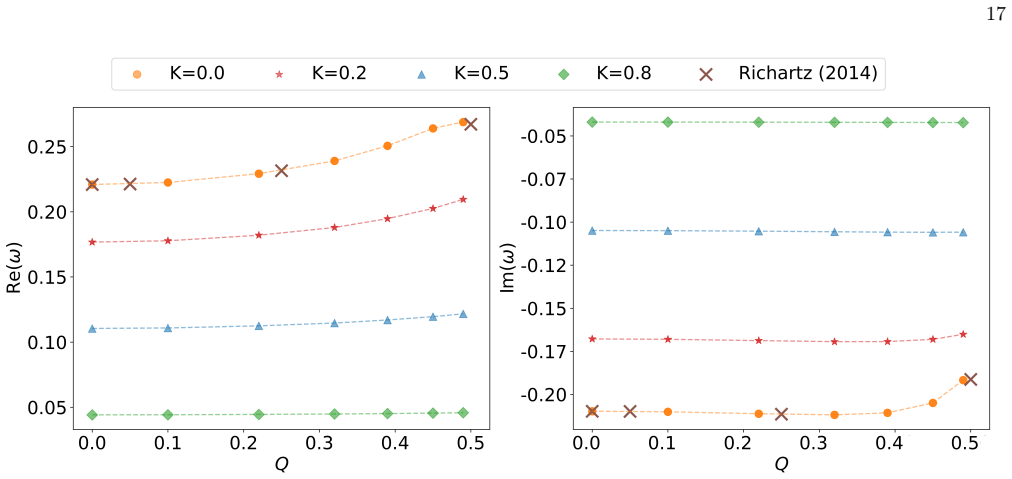
Dependence on the black-hole charge at fixed electrostatic interaction Here, we analyze the dependence of the QNM fre- quencies of a charged scalar field on the BH charge and fluid parameter, while keeping the electrostatic interac- tion fixed atqQ= 1. In this section, we focus on the fundamental, monopole mode and we present the higher multipolesl= 1,4in...
-
[3]
positive
Dependence on the electrostatic interaction at fixed black-hole charge Next, we investigate the dependence of the QNM fre- quencies on the electrostatic interaction,qQ, while keep- ing the BH charge fixed atQ= 0.05. We focus on the fundamental, monopole mode throughout this section. The results are shown in Fig. 8, where we display the real (left panel) a...
-
[4]
Application to the sixth-order WKB Approximation In the sixth-order WKB approximation, the quantity of interest is the right-hand side of Eq. (82). Here, we introduce it as the function W:= iU0q 2U(2) 0 −Λ 2 −Λ 3 −Λ 4 −Λ 5 −Λ 6 ,(D2) which is the combination of the WKB effective potential and its derivatives. We consider the parameter set {p}={Q, K, q, l}...
-
[5]
(D3) that is representative of our QNM computations with the WKB method, {q= 0.001, Q= 0.1, K= 0.5, l= 4}.(D5) We refer to this nominal tuple as tuple A in Fig
We begin by choosing a nominal tuple from the parameter set in Eq. (D3) that is representative of our QNM computations with the WKB method, {q= 0.001, Q= 0.1, K= 0.5, l= 4}.(D5) We refer to this nominal tuple as tuple A in Fig. 10. The valueK= 0.5is taken as the midpoint of the range considered in Case 1
-
[6]
(78) and the corresponding QNM frequencyω
For this nominal tuple, we compute the locationr0 of the maximum of the WKB effective potential in Eq. (78) and the corresponding QNM frequencyω
-
[7]
(D2) with respect toq,Q,K, andl, and we compute the sensitivity coefficients using Eq
We then calculate the partial derivatives of the functionWin Eq. (D2) with respect toq,Q,K, andl, and we compute the sensitivity coefficients using Eq. (D4). In this step,r0 andωare kept fixed at the values obtained in the previous step
-
[8]
Choosing representative values from this broader variation defines tuples B, C, and D in Fig
Next, we vary one of the continuous parameters,K, Q, orq, away from its nominal value while keeping the others fixed. Choosing representative values from this broader variation defines tuples B, C, and D in Fig. 10. They are given by B:{q= 0.001, Q= 0.1, K= 0.1, l= 4},(D6a) C:{q= 0.001, Q= 0.4, K= 0.5, l= 4},(D6b) D:{q= 10, Q= 0.1, K= 0.5, l= 4}.(D6c) For...
-
[9]
Error analysis for conventional root finder In Fig. 11 we present the absolute and relative errors of the fundamental, monopole QNM frequencies as func- tions of the truncation levelN, computed with conven- tional root finding algorithms. We show the errors in the real part of the frequency in the top panel, and the er- rors in the imaginary part in the b...
-
[10]
p f0 |qQ| r0 + √ 1−K r0 + 1 r3/2 0 !# ,(F7) and ωR = qQ r0 +O
Error Analysis for the Automatic Differentiation Implementation We repeat the truncation-error analysis for the imple- mentation based on Leaver’s continued fraction method combined with automatic differentiation introduced in Sec. IVC. To allow a direct comparison with the conven- tional root-finding implementation, we use the same BH and scalar-field pa...
2000
-
[11]
Uncharged Scalar Field For an uncharged scalar field,q= 0, the sixth-order WKB approximation reproduces the qualitative increase of the real part of the frequency with the BH chargeQ, in agreement with Leaver’s method. Fig. 13 shows excellent agreement between the two methods when the fluid pa- rameter vanishes (yellow dashed line). For example, for thel=...
-
[12]
As shown in Table VII and Fig
Charged Scalar Field Here we consider a charged scalar field and focus on the case where the interaction between charges isqQ= 1. As shown in Table VII and Fig. 14, the sixth-order WKB approximation continues to reproduce the qualitative de- pendence of the spectrum on the BH chargeQ, including the monotonic increase of the real part of the frequency alon...
-
[13]
N. Abacet al.(LIGO Scientific, VIRGO, KAGRA), GWTC-5.0: Observations from the Second Part of the Fourth LIGO-Virgo-KAGRA Observing Run and Updates to the Gravitational-Wave Transient Catalog (2026), arXiv:2605.27225 [gr-qc]
Pith/arXiv arXiv 2026
-
[14]
A. G. Abacet al.(LIGO Scientific, VIRGO, KA- GRA), GWTC-4.0: Updating the Gravitational-Wave Transient Catalog with Observations from the First PartoftheFourthLIGO-Virgo-KAGRAObservingRun (2025), arXiv:2508.18082 [gr-qc]
Pith/arXiv arXiv 2025
-
[15]
Abbottet al.(LIGO Scientific, Virgo, KAGRA), Astrophys
R. Abbottet al.(LIGO Scientific, Virgo, KAGRA), Astrophys. J.949, 76 (2023), arXiv:2111.03604 [astro- ph.CO]
Pith/arXiv arXiv 2023
-
[16]
B. P. Abbottet al.(LIGO Scientific, Virgo), Phys. Rev. Lett.116, 061102 (2016), arXiv:1602.03837 [gr-qc]
Pith/arXiv arXiv 2016
-
[17]
J. Badía and E. F. Eiroa, Phys. Rev. D102, 024066 (2020), arXiv:2005.03690 [gr-qc]
Pith/arXiv arXiv 2020
-
[18]
Ahmed, H
F. Ahmed, H. Ali, Q. Wu, T. Zhu, and S. G. Ghosh, Eur. Phys. J. C85, 795 (2025)
2025
-
[19]
A. Abdujabbarov, B. Toshmatov, Z. Stuchlík, and B. Ahmedov, Int. J. Mod. Phys. D26, 1750051 (2016), arXiv:1512.05206 [gr-qc]
Pith/arXiv arXiv 2016
-
[20]
H. Davoudiasl and P. B. Denton, Phys. Rev. Lett.123, 021102 (2019), arXiv:1904.09242 [astro-ph.CO]
Pith/arXiv arXiv 2019
-
[21]
P. V. P. Cunha, C. A. R. Herdeiro, and E. Radu, Uni- verse5, 220 (2019), arXiv:1909.08039 [gr-qc]
Pith/arXiv arXiv 2019
-
[22]
G. Creci, S. Vandoren, and H. Witek, Phys. Rev. D101, 124051 (2020), arXiv:2004.05178 [gr-qc]
Pith/arXiv arXiv 2020
-
[23]
J. C. Acevedo-Muñoz, F. D. Lora-Clavijo, and A. Cruz-Osorio, Phys. Rev. D111, 084022 (2025), arXiv:2503.22624 [gr-qc]
Pith/arXiv arXiv 2025
-
[24]
C. L. Ahmed Rizwan, A. Naveena Kumara, K. Hegde, M. S. Ali, and K. M. Ajith, Class. Quant. Grav.38, 075030 (2021), arXiv:2008.01426 [gr-qc]
Pith/arXiv arXiv 2021
-
[25]
B. Cuadros-Melgar, R. D. B. Fontana, and J. de Oliveira, Phys. Rev. D104, 104039 (2021), arXiv:2108.04864 [gr-qc]
Pith/arXiv arXiv 2021
-
[26]
H.-C. Kim, B.-H. Lee, W. Lee, and Y. Lee, Phys. Rev. D101, 064067 (2020), arXiv:1912.09709 [gr-qc]
Pith/arXiv arXiv 2020
-
[27]
B. Cuadros-Melgar, R. D. B. Fontana, and J. de Oliveira, Eur. Phys. J. C80, 848 (2020), arXiv:2003.00564 [gr-qc]
Pith/arXiv arXiv 2020
-
[28]
S. J. C., K. R., K. Hegde, K. M. Ajith, S. Punacha, and A. N. Kumara, Phys. Rev. D111, 064034 (2025), arXiv:2411.11629 [gr-qc]
Pith/arXiv arXiv 2025
-
[29]
C. A. Benavides-Gallego, A. A. Abdujabbarov, and C. Bambi, Phys. Rev. D101, 044038 (2020), arXiv:1811.01562 [gr-qc]
Pith/arXiv arXiv 2020
-
[30]
V. D. Ivashchuk, S. V. Bolokhov, F. B. Belis- sarova, N. Kydyrbay, A. N. Malybayev, G. S. Nur- bakova, and B. Zheng, Grav. Cosmol.31, 392 (2025), arXiv:2509.08465 [gr-qc]
Pith/arXiv arXiv 2025
-
[31]
V. Cardoso, I. P. Carucci, P. Pani, and T. P. Sotiriou, Phys. Rev. Lett.111, 111101 (2013), arXiv:1308.6587 [gr-qc]
Pith/arXiv arXiv 2013
-
[32]
L. Pezzella, K. Destounis, A. Maselli, and V. Cardoso, Phys. Rev. D111, 064026 (2025), arXiv:2412.18651 [gr- qc]
Pith/arXiv arXiv 2025
-
[33]
M. Alloqulov, A. Abdujabbarov, B. Ahmedov, and C. Yuan, Probing the gravity of a Schwarzschild black hole in the presence of a cloud of strings with EMRIs (2025), arXiv:2512.12672 [gr-qc]
arXiv 2025
-
[34]
S. Gliorio, E. Berti, A. Maselli, and N. Speeney, Phys. Rev. D112, 124050 (2025), arXiv:2503.16649 [gr-qc]
arXiv 2025
-
[35]
V. V. Kiselev, Class. Quant. Grav.20, 1187 (2003), arXiv:gr-qc/0210040
Pith/arXiv arXiv 2003
-
[36]
Z.-S. Qu, T. Wang, and C.-J. Feng, Eur. Phys. J. C83, 784 (2023), arXiv:2307.09079 [gr-qc]
Pith/arXiv arXiv 2023
-
[37]
A. Al-Badawi, F. Ahmed, and İ. Sakallı, Letelier black hole immersed in an electromagnetic universe (2025), arXiv:2512.00102 [gr-qc]
arXiv 2025
-
[38]
V. V. Kiselev, Quintessential solution of dark matter rotation curves and its simulation by extra dimensions (2003), arXiv:gr-qc/0303031
Pith/arXiv arXiv 2003
-
[39]
P. S. Letelier, Phys. Rev. D20, 1294 (1979)
1979
-
[40]
Vilenkin and E
A. Vilenkin and E. P. S. Shellard,Cosmic Strings and Other Topological Defects(Cambridge University Press, 2000)
2000
-
[41]
Vilenkin, Phys
A. Vilenkin, Phys. Rept.121, 263 (1985)
1985
-
[42]
Barriola and A
M. Barriola and A. Vilenkin, Phys. Rev. Lett.63, 341 (1989)
1989
-
[43]
Harari and C
D. Harari and C. Lousto, Phys. Rev. D42, 2626 (1990)
1990
-
[44]
K. Freese, EAS Publ. Ser.36, 113 (2009), arXiv:0812.4005 [astro-ph]
Pith/arXiv arXiv 2009
-
[45]
F. Rahaman, P. K. F. Kuhfittig, K. Chakraborty, M. Kalam, and D. Hossain, Int. J. Theor. Phys.50, 2655 (2011), arXiv:1101.2515 [gr-qc]
Pith/arXiv arXiv 2011
- [46]
-
[47]
Kalb and P
M. Kalb and P. Ramond, Phys. Rev. D9, 2273 (1974)
1974
-
[48]
P. S. Letelier, Phys. Rev. D15, 1055 (1977)
1977
-
[49]
Vilenkin, Phys
A. Vilenkin, Phys. Rev. D23, 852 (1981)
1981
-
[50]
C. V. Vishveshwara, Nature227, 936 (1970)
1970
-
[51]
K. D. Kokkotas and B. G. Schmidt, Living Rev. Rel.2, 2 (1999), arXiv:gr-qc/9909058
Pith/arXiv arXiv 1999
-
[52]
E. Berti, V. Cardoso, and A. O. Starinets, Class. Quant. Grav.26, 163001 (2009), arXiv:0905.2975 [gr-qc]
Pith/arXiv arXiv 2009
-
[53]
Bertiet al., Black hole spectroscopy: from theory to experiment (2025), arXiv:2505.23895 [gr-qc]
E. Bertiet al., Black hole spectroscopy: from theory to experiment (2025), arXiv:2505.23895 [gr-qc]
Pith/arXiv arXiv 2025
-
[54]
R. A. Konoplya and A. Zhidenko, Rev. Mod. Phys.83, 793 (2011), arXiv:1102.4014 [gr-qc]
Pith/arXiv arXiv 2011
-
[55]
N. Varghese and V. C. Kuriakose, Mod. Phys. Lett. A 29, 1450113 (2014), arXiv:1407.6292 [gr-qc]
Pith/arXiv arXiv 2014
-
[56]
Y. Zhang, Y. X. Gui, and F. Li, Gen. Rel. Grav.39, 1003 (2007), arXiv:gr-qc/0612010
Pith/arXiv arXiv 2007
-
[57]
C. Ma, Y. Gui, W. Wang, and F. Wang, Central Eur. J. Phys.6, 194 (2008), arXiv:gr-qc/0611146
Pith/arXiv arXiv 2008
-
[58]
S.-b. Chen and J.-l. Jing, Class. Quant. Grav.22, 4651 (2005), arXiv:gr-qc/0511085
Pith/arXiv arXiv 2005
-
[59]
E. W. Leaver, Proc. Roy. Soc. Lond. A402, 285 (1985)
1985
-
[60]
E. W. Leaver, Phys. Rev. D41, 2986 (1990)
1990
-
[61]
Kopteva, J
E. Kopteva, J. Zhang, D. N. Garzon, H. Da Silva, and H. Witek (2026), in preparation
2026
-
[62]
U. Nucamendi and D. Sudarsky, Class. Quant. Grav. 14, 1309 (1997), arXiv:gr-qc/9611043
Pith/arXiv arXiv 1997
-
[63]
I. D. Novikov, General Relativity and Gravitation33, 2259 (2001)
2001
-
[64]
C. W. Misner, K. S. Thorne, and J. A. Wheeler,Grav- itation(W. H. Freeman, San Francisco, 1973)
1973
-
[65]
V. P. Frolov and I. D. Novikov, eds.,Black hole physics: Basic concepts and new developments(1998)
1998
-
[66]
M. Dafermos and J. Luk, Ann. Math. (2)202, 309 34 (2025), arXiv:1710.01722 [gr-qc]
arXiv 2025
-
[67]
M. Van de Moortel, Asymptotically flat black holes with a singular Cauchy horizon and a spacelike singularity (2025), arXiv:2510.07431 [gr-qc]
arXiv 2025
-
[68]
J. D. Brown, J. Creighton, and R. B. Mann, Phys. Rev. D50, 6394 (1994), arXiv:gr-qc/9405007
Pith/arXiv arXiv 1994
- [69]
-
[70]
C. A. R. Herdeiro, J. C. Degollado, and H. F. Rúnars- son, Phys. Rev. D88, 063003 (2013), arXiv:1305.5513 [gr-qc]
Pith/arXiv arXiv 2013
-
[71]
S. R. Dolan, S. Ponglertsakul, and E. Winstanley, Phys. Rev. D92, 124047 (2015), arXiv:1507.02156 [gr-qc]
Pith/arXiv arXiv 2015
-
[72]
O. J. C. Dias and R. Masachs, Class. Quant. Grav.35, 184001 (2018), arXiv:1801.10176 [gr-qc]
Pith/arXiv arXiv 2018
-
[73]
Senjaya, Phys
D. Senjaya, Phys. Lett. B848, 138373 (2024), published online Dec 2023
2024
-
[74]
N. Sanchis-Gual, A. Belchí, C. Herdeiro, and J. A. Font, Reducing the irreducible: the charged black hole bomb in a moving cavity (2025), arXiv:2506.06527 [gr-qc]
Pith/arXiv arXiv 2025
-
[75]
B.-W. Qin and Y.-P. Zhang, Phys. Rev. D113, 124070 (2026), arXiv:2602.05268 [gr-qc]
arXiv 2026
-
[76]
G. B. Arfken and H. J. Weber,Mathematical Methods for Physicists, 6th ed. (Elsevier Academic Press, Ams- terdam, 2005)
2005
-
[77]
W. G. Baber and H. R. Hassé, Math. Proc. Camb. Phil. Soc.31, 564 (1935)
1935
-
[78]
A. H. Wilson, Proc. R. Soc. Lond. A118, 617 (1928)
1928
-
[79]
Griewank, Acta Numerica12, 321 (2003)
A. Griewank, Acta Numerica12, 321 (2003)
2003
-
[80]
D. C. Liu and J. Nocedal, Math. Program.45, 503 (1989)
1989
discussion (0)
Sign in with ORCID, Apple, or X to comment. Anyone can read and Pith papers without signing in.