REVIEW 2 major objections 4 minor 175 references
This paper claims that classical and quantum semiparametric efficiency are the same Hilbert-space theorem, and that the channel version makes imaging limits and SPADE's advantage computable.
Reviewed by Pith at T0; open to challenge. T0 means a machine referee read the full paper against a public rubric. the ladder, T0–T4 →
T0 review · deepseek-v4-flash
2026-08-01 07:09 UTC pith:5WKZFBWS
load-bearing objection A competent, largely rigorous unification of classical and quantum semiparametric efficiency; the imaging numerics rest on an unproven but likely fixable compactness assumption. the 2 major comments →
Unified theory of classical and quantum semiparametric efficiency
The pith
A machine-rendered reading of the paper's core claim, the machinery that carries it, and where it could break.
Core claim
The central claim is that the semiparametric efficiency bound is always the squared norm of a single object, the efficient influence. Perturbations of the unknown parameter are represented as tangent vectors, each pushed forward to a 'score' in an ambient Hilbert space whose inner product is the Fisher or Helstrom information. If the parameter of interest is differentiable and its score differential is bounded, the Riesz representation theorem gives a unique efficient influence whose squared norm is exactly the bound (Theorem 2.1). Through a channel, the output efficient influence is the pseudo-inverse of the channel pullback applied to the input efficient influence (Theorem 4.1), so channel
What carries the argument
The carrying object is the score tangent space: a Hilbert space formed by pushing tangent vectors of the parameter manifold into an ambient space of scores, with inner product given by the Fisher or Helstrom information. The efficient influence is the Riesz representative of the score differential, and the efficiency bound is its squared norm. For channels, three local maps do the work: the channel pushforward, its adjoint pullback, and the information map formed by composing them. Their singular value decomposition gives the singular values and vectors used to compute output bounds and to compare measurements such as direct imaging and SPADE.
Load-bearing premise
The singular-value sums that produce the numerical imaging bounds assume the channel's linearized response can be decomposed into discrete components whose sizes shrink fast enough to sum; the paper says in an appendix that it has not proved this for the imaging channels.
What would settle it
For a given point-spread function and object size, compute the singular value decomposition of the discretized channel pushforward at increasing resolution and check whether the sum of squared singular values and the efficiency bound for a fixed coefficient converge; if the truncated sums grow without bound as resolution increases, the singular-value formulas are not justified.
If this is right
- For any semiparametric model, computing the efficiency bound reduces to solving a Riesz-representation problem in a score Hilbert space, rather than analyzing estimators case by case.
- Through a channel, the output efficient influence is obtained by pseudo-inverting the channel pullback, so channel effects on fundamental error limits become linear algebra.
- Channels without access to the parameter are monotonic: they cannot decrease the efficiency bound, confirming the data-processing intuition.
- For Gaussian and Poisson fields the theory simplifies to weighted Hilbert-space calculus, making infinite-dimensional imaging limits numerically computable via SVD.
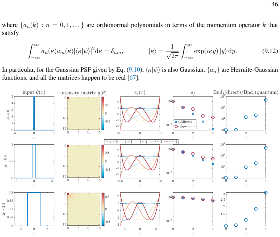
- For subdiffraction incoherent imaging, direct imaging has much larger bounds than the quantum limits for estimating high-order Fourier-type coefficients, while spatial-mode demultiplexing substantially closes the gap.
Where Pith is reading between the lines
- Editorial inference: If the compactness gap is filled, the same SVD machinery becomes a general numerical recipe for any sensor, allowing semiparametric bounds and near-optimal measurements to be computed without model-specific derivations.
- Editorial inference: The unresolved compactness of the channel pushforward suggests a concrete program: prove or disprove trace-class behavior for physical point-spread functions, and if compactness fails, examine whether finite-rank truncations still approximate the bound with controlled error.
- Editorial inference: Structured illumination problems such as confocal microscopy enter as direct sums of channels, so the additivity of information maps implies illumination patterns can be optimized as a broadcast-channel design problem.
- Editorial inference: The one-step estimator construction points toward adaptive hardware: a preliminary estimate programs the efficient-influence measurement, connecting semiparametric efficiency to programmable interferometers.
Editorial analysis
A structured set of objections, weighed in public.
Referee Report
Summary. The paper claims a unified semiparametric efficiency theory for classical and quantum statistics, extending Cramér-Rao and Helstrom bounds to infinite-dimensional parameters. Abstractly, a model is represented by a tangent space, a pushforward map, and an information inner product; the semiparametric bound is the squared norm of the Riesz representative (efficient influence) of the score differential (Theorem 2.1). For channels, the output efficient influence is the pseudo-inverse of the channel pullback applied to the input influence (Theorem 4.1), with a bound expressible via the information map. The framework is illustrated on classical, Poisson, Gaussian, quantum, quantum-Poisson, and quantum-Gaussian models, and applied to coherent and incoherent imaging, with SVD-based numerical bounds for direct imaging and SPADE. The paper includes extensive proofs and an appendix explicitly listing unproved regularity and compactness conditions.
Significance. The abstract theorems are elegant and appear correct within their stated assumptions. Theorem 4.1 generalizes finite-dimensional pseudo-inverse formulas and provides a principled way to compute channel-degraded bounds. The information-map additivity for broadcast channels is a nice result. The paper's main strength is the unification and geometric perspective, which should be useful for future applications. The manuscript is also unusually transparent: Appendix J admits the compactness and regularity gaps. The validation against a prior submodel method (Fig. 19) adds confidence in the pseudo-inverse implementation. However, the quantitative imaging claims are not yet rigorous because they depend on unproved SVD convergence; this prevents acceptance in current form.
major comments (2)
- [Secs. 4 G, 7–10; Appendix J, item 6] The SVD expansions used for the quantitative bounds—Eqs. (4.66), (7.24), (8.17), and the SPADE comparisons in Sec. 10—presuppose that the channel pushforward F_push is compact. Appendix J item 6 concedes that compactness is not proved for any channel in Secs. 7–10 and that convergence of finite-rank truncations is open. The unqualified claim in the abstract that SPADE 'can be far superior' is based on these truncations. For the Gaussian-PSF direct-imaging channel (Eq. 8.20), after the weighted-norm unitary transformation, the kernel is F(y|x)√θ(x)/√g(y); the paper gives no proof that this kernel defines a compact operator, and if compactness fails the infinite sums in Eqs. (4.66)/(8.17) need not converge to the true bound. The authors should either prove compactness/approximation for the studied channels or explicitly mark all SVD-based numerical bounds as heuristic and remove or qualify
- [Secs. 3 B–3 D; Appendix J, items 1–2] The nonparametric quantum and quantum-Poisson results (∇β=b−⟨b,I⟩θ I in Eq. 3.24 and ∇β=b in Eq. 3.27) depend on maximality of the score tangent space. Appendix J items 1–2 state that the classical differentiability-in-quadratic-mean condition is not yet extended to these models and that the infinite-dimensional Poisson/Gaussian quantum results may be less rigorous. Because Secs. 9–10 build on these maximality assumptions, the imaging bounds are conditional on regularity conditions that are not stated in the main text. The main text should state these conditions, or at least clearly flag the formal nature of the nonparametric models, before drawing quantitative conclusions.
minor comments (4)
- [Fig. 17 caption] The caption says 'the same as those of Fig. 17' but should refer to Fig. 16.
- [Eq. (10.1)] The polynomial p_j(x) is defined with the sum starting at k=1, omitting a possible constant term. Clarify the convention for j=0 and the relationship to the moments {γ_k}.
- [Appendix G] The text asserts that the chosen discretizations have 'minimal effects' but provides no convergence study. Given the open compactness question, a short numerical convergence check (e.g., singular values versus grid size or mode dimension) would substantially strengthen the numerical claims.
- [Sec. 8 D, Eq. (8.7)] For the sinc² PSF in Eq. (8.23), g(θ,y) can vanish at isolated points, making the division by g(θ,y) in Eq. (8.7) delicate. The quotient-space construction handles null sets formally, but the numerical implementation should state how zeros are treated.
Circularity Check
No load-bearing circular reduction found; the central bounds are derived in-text from definitions, with self-citations and the compactness caveat as non-circular limitations.
full rationale
Walking the derivation chain: Bnd(θ) is defined in Eq. (2.46) as a supremum over submodel bounds, and Theorem 2.1 identifies it with the squared norm of the Riesz representative of the score differential. This is a direct Hilbert-space argument from the definition, not a fitted input or a self-referential construction. Theorem 4.1 derives the output efficient influence as the pseudo-inverse of the channel pullback by solving F_pull ∇outβ = ∇β, obtained from the adjoint relation (4.28); again, this is a proof from the stated mathematical objects. The SVD expansions in Eqs. (4.66), (7.24), and (8.17) are explicitly conditional on compactness, and Appendix J.6 admits that compactness of F_push is unproved for all channels in Secs. 7–10 and that finite-rank convergence is open. That is a genuine mathematical gap limiting the rigor of the numerical SVD-based bounds, but it is not circularity: no equation is assumed that is equivalent to the conclusion, and no parameter is fitted to make the reported bounds match a target. The paper does contain many self-citations ([9] for quantum semiparametric estimation, [30] for Poisson states, [44] for SPADE), but these supply background models, technical lemmas, or previously proposed measurement schemes; the central abstract derivation and the channel-transformation theorem do not reduce to those citations. The validation against Ref. [12] in Fig. 19 is a cross-check between two numerical methods, not a fitted input to the derivation. Under the required quote-and-reduction standard, no specific circular step can be exhibited.
Axiom & Free-Parameter Ledger
free parameters (2)
- Mode-space dimension for quantum channel SVD =
16
- Numerical discretization steps Δx, Δy =
Δ/100 to Δ/500 and Δ_out/500 to Δ_out/1000
axioms (5)
- standard math Riesz representation theorem
- ad hoc to paper Compactness of the channel pushforward F_push
- domain assumption Poisson-state approximation of thermal/incoherent light
- domain assumption Regular estimator / local asymptotic conditions
- domain assumption Maximality of score tangent space for nonparametric models
read the original abstract
In classical and quantum statistics, high-dimensional unknown parameters are abundant and it is often prudent to make minimal assumptions about them using so-called semiparametric models. To attack a wide range of semiparametric problems in one broad stroke, we present a unified treatment of statistical efficiency for classical and quantum semiparametric models, generalizing the Cram\'er-Rao and Helstrom bounds beyond finite-dimensional parameters. We introduce the fundamental concepts in abstract and geometric terms before applying them to many examples, covering general classical and quantum models as well as the paradigmatic special cases of Gaussian and Poisson fields. We give an in-depth treatment of channels in the semiparametric efficiency theory and advocate the use of the singular value decomposition to elucidate the statistical effects of channels. To demonstrate the utility of the formalism, we apply it to coherent and incoherent optical imaging problems, assuming an arbitrary field or intensity on the object plane without parametric assumptions. Our formalism enables us to compute classical and quantum limits to coherent and incoherent imaging resolution in statistical terms. For subdiffraction incoherent imaging, we demonstrate that spatial-mode demultiplexing can be far superior to direct imaging in estimating generalized Fourier coefficients and come closer to the quantum limits. We envision our theory becoming an essential tool for both classical and quantum statistics with useful applications to sensing and imaging, whenever minimal assumptions about a high-dimensional parameter should be made.
Figures




Reference graph
Works this paper leans on
-
[1]
Many more semiparametric problems can be found in the classical statistics literature [1–6] and may be generalizable to quantum problems. One notable omission in this work is a treatment of explicit nuisance parameters, which is a vast subject in classical statistics and has seen some studies in the quantum arena as well [9, 97]
-
[2]
This work focuses on parameters of interest that are linear functionals of the underlying parameter, but the general theory can also be applied to nonlinear functionals, such as the entropy of a probability density or density operator [2, 9]
-
[3]
The classical and quantum Gaussian models in Examples 2.3 and 2.6 assume that the covariance maps are given. The models can be generalized for unknown covariance maps [52, 53, 58] or unknown power spectral densities for stationary processes [98–101] by generalizing the score vector spaces and the semi-inner products
-
[4]
The implementations require more studies, especially for quantum problems where the physical processing layer is experimentally nontrivial
When the efficient influence is parameter-dependent, we suggest only one-step estimators and gloss over the details of their implementations. The implementations require more studies, especially for quantum problems where the physical processing layer is experimentally nontrivial. 53
-
[5]
5 B should find many more applications in sensing and imaging beyond the example of structured illuminations in Sec
The theory of broadcast channels in Sec. 5 B should find many more applications in sensing and imaging beyond the example of structured illuminations in Sec. 11, any time scanning, multiple probes, multiple apertures, or multiple modalities are employed to observe the same sample [25, 102]
-
[6]
These limitations are especially detrimental to the problem of reconstructing a functional parameterθ, for which a Bayesian or minimax framework may be more appropriate [103–108]
The efficiency theory is limited by its regularity assumptions, its reliance on asymptotics, and its inability to incorporate prior information. These limitations are especially detrimental to the problem of reconstructing a functional parameterθ, for which a Bayesian or minimax framework may be more appropriate [103–108]. A transition to those frameworks...
-
[7]
8–11, we consider only measurements that produce Poisson fields
In our study of incoherent imaging in Secs. 8–11, we consider only measurements that produce Poisson fields. It is possible to model more general measurements that produce non-Poisson fields, such as homodyne or heterodyne detection, by returning to the quantum state of optical field from which the Poisson state is derived. However, such measurements must...
-
[8]
Roy Pike,The Limits of Resolution(CRC Press, Boca Raton, 2016)
Geoffrey de Villiers and E. Roy Pike,The Limits of Resolution(CRC Press, Boca Raton, 2016)
2016
-
[9]
Quantum Semiparametric Estimation,
Mankei Tsang, Francesco Albarelli, and Animesh Datta, “Quantum Semiparametric Estimation,” Physical Review X10, 031023 (2020)
2020
-
[10]
In general, we call an operator on a vector space amapto avoid confusion with the quantum operators
We reserve the termoperatorfor an operator on a complex Hilbert space in quantum mechanics. In general, we call an operator on a vector space amapto avoid confusion with the quantum operators. The operator norm of a map is still called the operator norm, however. 2.Idenotes the identity map; it may be the identity operator, the identity map, or the identi...
-
[11]
We focus on the incoherent case
INCOHERENT IMAGING WITH STRUCTURED ILLUMINATIONS Our formalism can handle structured illuminations [40], such as confocal microscopy, just as well. We focus on the incoherent case. Fig. 18 illustrates the setup. Suppose that the illumination intensity pattern changes overJtime intervals. Leth j(x)be the illumination intensity in thejth time interval. The ...
-
[12]
We highlight some of them in the following:
POTENTIAL EXTENSIONS Despite the length of this work, it introduces only a framework of the semiparametric efficiency theory and begets many more open questions. We highlight some of them in the following:
-
[13]
Perturbations of a parameter are represented by tangent vectors
CONCLUSION The essence of the semiparametric efficiency theory is geometric. Perturbations of a parameter are represented by tangent vectors. The vectors are endowed with statistically motivated metrics. The infinite dimensionality of the parameter space is handled by treating the tangent vectors in Hilbert spaces. The parameter of interest as well as the...
2024
-
[14]
A∗ of a Banach-space mapAdenotes its dual.A ∗ of a Hilbert-space mapAdenotes its adjoint
For a vector spaceV,V ∗ denotes its dual, a space of linear functionals of vectors, also called covectors. A∗ of a Banach-space mapAdenotes its dual.A ∗ of a Hilbert-space mapAdenotes its adjoint. We also use†to denote the adjoint when the Hilbert spaces are different from those for∗. For a matrix A, (a)A ∗ denotes the conjugate transpose, (b)A ⊤ denotes ...
-
[15]
If a proof is not given immediately after a numbered proposition and no reference is provided, the proof is delegated to Appendix I
-
[16]
Symbol Definition First mention θparameter Sec
Table I provides a list of symbols. Symbol Definition First mention θparameter Sec. 2 A Θparameter space Sec. 2 A ϕparametric submodel Sec. 2 A ˙ϕdirectional derivative Sec. 2 A Tθ tangent space atθSec. 2 A β(θ)parameter of interest Sec. 2 A dβ( ˙ϕ)differential ofβSec. 2 A bndθ( ˙ϕ)submodel efficiency bound Sec. 2 B infoθ( ˙ϕ,˙χ)information semimetric Sec...
-
[17]
An important concept is a pure quantum state|α⟩ ∈Γ(H)called the coherent state, withα∈ Hmodeling the mean field.|0⟩is the vacuum state
Bosonic Fock space LetΓ(H)be the bosonic Fock space constructed from a complex mode Hilbert spaceH[56].Γ(H)is a complex Hilbert space itself; we use the bra-ket notation with it. An important concept is a pure quantum state|α⟩ ∈Γ(H)called the coherent state, withα∈ Hmodeling the mean field.|0⟩is the vacuum state. The linear span of{|α⟩:α∈ H}is a dense sub...
-
[18]
Phase space To conform with the classical treatment in Example 2.3, where all spaces are real, we now transform the complexHto a real Hilbert spaceKusing a procedure called realification [115].Kis called the phase space in physics. LetC:H → Hbe an antiunitary conjugation map satisfying ⟨α, γ⟩H =⟨Cγ,Cα⟩ H ∀α, γ∈ H,C 2 =I.(B10) Such a map always exists—we c...
-
[19]
Let the phase space be the real Hilbert space K=RH ⊕IH.(B17) The inner product is defined as A′ ⊕A ′′, B′ ⊕B ′′ K = A′, B′ H + A′′, B′′ H .(B18) It is often convenient to write each element ofKin the block form A=A ′ ⊕A ′′ = A′ A′′ .(B19)
-
[20]
The inverse ofUcan be expressed as U −1A=U −1 A′ A′′ = 1i A′ A′′ =A ′ +iA ′′.(B23)
Define the mapU:H → Kas U α=Rα⊕Iα= R I α,(B20) 58 such thatK=UHandUis surjective.Uis called the realification map.Uis isometric in the sense of Re⟨α, γ⟩H =⟨U α, U γ⟩K ,(B21) ∥α∥H =∥U α∥K,(B22) butUis not a unitary map in the conventional sense, becauseHis complex whileKis real. The inverse ofUcan be expressed as U −1A=U −1 A′ A′′ = 1i A′ A′′ =A ′ +iA ′′.(B23)
-
[21]
In block form, J= 0−I I0 .(B26)
Let the complex-structure mapJ:K → Kbe J(A ′ ⊕A ′′) = (−A′′)⊕A ′,(B24) such that Im⟨α, γ⟩H =− ⟨U α, J U γ⟩K , J ∗ =−J, J 2 =−I,(B25) where∗of a matrix denotes the conjugate transpose. In block form, J= 0−I I0 .(B26)
-
[22]
Let the modal quadrature observables onΓ(H)in terms of a phase-space vectorA∈ Kbe P(A) =p(U −1A), X(A) =q(U −1A) =P(−J A).(B27) P(A) =X(J A)andX(A)are both linear with respect toAby virtue of Eqs. (B5). The canonical commutation relations become [X(A), P(B)]|η⟩=i⟨A, B⟩ K |η⟩,[X(A), X(B)]|η⟩=−i⟨A, J B⟩ K |η⟩.(B28)
-
[23]
Let the phase-space displacement operatorW(A)onΓ(H)in terms ofA∈ Kbe W(A) = exp[−iP(A)] =D(U −1A/ √ 2).(B29) A convenient formula is W(B) ∗eiX(A) W(B) =e i⟨A,B⟩KeiX(A) .(B30) Now the quadrature observableX(A)of the mode specified byA∈ Kis a more precise generalization of the random variableL(X)withL∈ B ∗ in Example 2.3. 59
-
[24]
Gaussian states When the mode spaceHis infinite-dimensional, the literature does not seem to offer any general definition of the covariance mapΣon the phase spaceK, Gaussian states on the bosonic Fock spaceΓ(H), or Gaussian channels, so we write down some formal expressions that are correct at least in the finite-dimensional case [29], while adopting nota...
-
[25]
An estimator ˇβ: Ω→R is called unbiased if Eθ ˇβ−β(θ) = Z ˇβ(ω)−β(θ) f(θ, ω)dµ(ω) = 0∀θ∈Θ.(C1) A mathematically weaker condition called local unbiasedness follows if Eq
Unbiased estimators Let{f(θ,·) :θ∈Θ}be a set of probability densities, following Example 2.1. An estimator ˇβ: Ω→R is called unbiased if Eθ ˇβ−β(θ) = Z ˇβ(ω)−β(θ) f(θ, ω)dµ(ω) = 0∀θ∈Θ.(C1) A mathematically weaker condition called local unbiasedness follows if Eq. (C1) holds at the true parameter valueθand also ˙ϕE θ ˇβ−β(θ) = 0∀ ˙ϕ∈ Tθ (C2) at the trueθ. ...
-
[26]
To truly relax the conditions, one way is to consider a sequence of observations and appeal to asymptotics [1]
Regular estimators Since the estimator is not supposed to know the true parameter, local unbiasedness is hardly a relaxation of the global condition in practice and many estimators do not satisfy the conditions; even the maximum- likelihood estimator may be biased—locally and globally—and violate the efficiency bound [1, 116]. To truly relax the condition...
-
[27]
The resulty ′ is inrangeT
Null the component ofyin(rangeT) ⊥. The resulty ′ is inrangeT
-
[28]
Sincey ′ ∈rangeT, a solutionx∈domainT=H 1 always exists
SolveT x=y ′. Sincey ′ ∈rangeT, a solutionx∈domainT=H 1 always exists. Given a solution x, any other solution is in the formx+zfor somez∈kernelT
-
[29]
In this work, all the arguments ofT − are inrangeT(or else we set the output to be∞essentially), so the first step is never involved
Output the solutionx ′ with minimum norm ∥x′∥= inf x∈H1:T x=y′ ∥x∥.(D7) This solutionx ′ is unique and in(kernelT) ⊥. In this work, all the arguments ofT − are inrangeT(or else we set the output to be∞essentially), so the first step is never involved. The second and final steps are the essential operations in our use of the pseudo-inverse. It follows that...
-
[30]
The minimization is achieved whenK={0}andK ⊥ =H 1 forj= 0and K= span{e 0,
Min-max characterization: sj(T) = min K:dimK=j max x∈K⊥,∥x∥=1 ∥T x∥,(E1) In other words, for anyjth-dimensional subspaceKofH 1,s j ≤max x∈K⊥,∥x∥=1 ∥T x∥for the orthocomplementK ⊥. The minimization is achieved whenK={0}andK ⊥ =H 1 forj= 0and K= span{e 0, . . . , ej−1}forj≥1
-
[31]
For any compactTand any boundedT ′, sj T ′T ≤ T ′ sj(T), s j T T′ ≤s j(T) T ′ .(E2)
LetT ′ be another bounded Hilbert-space map (∥T ′∥<∞) with appropriate domain and codomain. For any compactTand any boundedT ′, sj T ′T ≤ T ′ sj(T), s j T T′ ≤s j(T) T ′ .(E2)
-
[32]
, N}be a set of vector spaces
If both maps are compact, sj+k T ′T ≤s j T ′ sk(T), s j+k (T+T ′)≤s j(T) +s k(T ′).(E3) Appendix F: Direct sum of vector spaces Let{V j :j= 1,2, . . . , N}be a set of vector spaces. The direct sumW=⊕ jVj is the vector space where each element is written as⊕ jAj withA j ∈ Vj.⊕ j is assumed to be linear, that is, c M j Aj = M j cAj,∀c∈RorC, M j Aj + M j Bj ...
-
[33]
Similarly, approximate each vector inA(g)by a concrete representation in a finite- dimensionalH 2
Approximate each abstract vector inA(f)by a concrete representation in a finite-dimensional vector spaceH 1. Similarly, approximate each vector inA(g)by a concrete representation in a finite- dimensionalH 2
-
[34]
Define inner products forH 1,2 to approximate the inner products forA(f)andA(g)
-
[35]
Convert the representations inH 1,2 to Euclidean vectors inH I,II via operatorsU:H 1 →H I and V:H 2 →H II , such that the inner products forH 1,2 coincide with the Euclidean inner products for HI,II
-
[36]
GivenU:H 1 →H I andV:H 2 →H II , abstract maps onA(f)andA(g)can be converted to matrices onH I,II
-
[37]
In particular, the Euclidean pseudo-inverse is the Moore–Penrose inverse
Given the Euclidean vectors inH I,II and the matrices onH I,II , the linear algebra can be computed numerically using standard routines. In particular, the Euclidean pseudo-inverse is the Moore–Penrose inverse
-
[38]
The following proposition summarizes the basic facts about the conversions
Convert the Euclidean vectorsV∇ outβ,{U ej}, and{V oj}inH I,II back to the original representa- tions inH 1,2 viaU −1 andV −1 if necessary, for plotting for example. The following proposition summarizes the basic facts about the conversions. 66 Proposition G.1.LetH j be a Hilbert space with inner product⟨·,·⟩ j.H 1 andH I are isomorphic if and only if the...
-
[39]
7 E, each vector in the inputVis a functionA(x)ofx∈D= [−∆,∆]
Classical coherent imaging In Sec. 7 E, each vector in the inputVis a functionA(x)ofx∈D= [−∆,∆]. An obvious and intuitive finite-dimensional representation ofA(x)is then A= A(x1) A(x2) ... ∈H 1, x j =x 0 +j∆x.(G17) The inner product can be approximated as ⟨A, B⟩f = Z D A(x)B(x)dx≈ X j A(xj)B(xj)∆x.(G18) To convertA∈H 1 to a EuclideanU A∈H I thro...
-
[40]
8 D, each vector inVis a functionA(x)ofx∈D= [−∆,∆]
Direct incoherent imaging In Sec. 8 D, each vector inVis a functionA(x)ofx∈D= [−∆,∆]. Assume the representation given by Eqs. (G17). The inner product in Eqs. (H27) can be approximated as ⟨A, B⟩θ ≈ X j A(xj)B(xj)θ(xj)∆x.(G23) The Euclidean versionU A∈H I should then be defined as (U A)j = q θ(xj)∆xA(xj).(G24) Similarly, for each functionA(y)inV out, assum...
-
[41]
Quantum channel Consider the quantum channel in Example 4.4. Diagonalizing the input density operator as f= X j λj |j⟩ ⟨j|,(G28) and taking the complex matrix representation of an operatorAas Ajk =⟨j|A|k⟩(G29) in terms of the eigenvectors off, the complex operator inner product can be approximated as the finite sum [57] tr [f(A∗ ⋆ B)]≈ X jk λj +λ k 2 Ajk ...
-
[42]
9 B, the classical-quantum channel given by Eq
Quantum model of incoherent imaging In Sec. 9 B, the classical-quantum channel given by Eq. (9.1) is studied. Assuming Eqs. (G23) and (G24) for the input spaces and Eqs. (G42) for the output spaces, the Markov-map dual given by Eq. (9.5) can be expressed as (F ∗A)µ = X j′k′ (F ∗)µ,j′k′Aj′k′,(F ∗)µ,j′k′ =⟨ψ|e ikxµ j′ k′ e−ikxµ |ψ⟩,(G46) which is a special ...
-
[43]
10, SPADE for incoherent imaging as per Eqs
Spatial-mode demultiplexing (SPADE) for incoherent imaging In Sec. 10, SPADE for incoherent imaging as per Eqs. (10.2)–(10.5) is studied. Assume Eqs. (G23) and (G24) for the input spaces. For the output spaces, let A= A(1,0) A(1,1) ... A(2,0) A(2,1) ... ∈H 2,(V A) τ n= p g(θ, τ, n)A(τ, n),(G48) treating(τ, n)as one index for a vect...
-
[44]
3 E and Sec
Hilbert spaces We follow the quantum Gaussian models in Examples 2.6 and 4.6 as well as Secs. 3 E and Sec. 6 C. Let the mode spaceHfor a paraxial quasimonochromatic field of one polarization be the space of complex functions on the object planeD⊆R m with inner product ⟨α, γ⟩H = Z D α(x)γ(x)dmx.(H1) Eachα∈ Hspecifies a spatiotemporal mode on the object pla...
-
[45]
It is a Gaussian channel [29]
Coherent states Assume that the imaging system comprises passive linear optics and a zero-temperature environment. It is a Gaussian channel [29]. Let us first consider a coherent state|α⟩ ∈Γ(H)for the input. The output state turns out to be a coherent state|γ⟩ ∈Γ(Hout)as well [120]. A linear mapS:H → Hout relates the input mean fieldα∈ Hto the output mean...
-
[46]
Then the channel mapsSandFfor the mean fields as well as the noise covariance mapΣ noise should all remain the same
Gaussian states Now consider an arbitrary Gaussian input state specified by a certain covariance mapΣ, and suppose that the channel remains the same. Then the channel mapsSandFfor the mean fields as well as the noise covariance mapΣ noise should all remain the same. To deriveΣ noise, we combine Eqs. (4.13) and (H26) for coherent states to obtain Σnoise = ...
-
[47]
7 D in the classical case, scaling coefficients in the quantum case must respect physics and thus require more care to model
Scaling Unlike Sec. 7 D in the classical case, scaling coefficients in the quantum case must respect physics and thus require more care to model. Three types of scaling at different stages of the system are possible:
-
[48]
Then score( ˙ϕ, c1) =c 1 ˙ϕ(θ) = score( ˙ϕ,1),(∇β)(·, c 1) = 1 c1 (∇β)(·,1),(H39) (∇outβ)(·, c1) = 1 c1 (∇outβ)(·,1),Bnd out(·, c1) = 1 c2 1 Bndout(·,1).(H40)
If the input mean fieldf(θ)is scaled by a given constantc 1 >0, it can be modeled by assuming f(θ, c1) =c 1θ,(H38) while the unknown parametersθandβ(θ)remain fixed for anyc 1. Then score( ˙ϕ, c1) =c 1 ˙ϕ(θ) = score( ˙ϕ,1),(∇β)(·, c 1) = 1 c1 (∇β)(·,1),(H39) (∇outβ)(·, c1) = 1 c1 (∇outβ)(·,1),Bnd out(·, c1) = 1 c2 1 Bndout(·,1).(H40)
-
[49]
Suppose thatF(c 2)has been confirmed to be monotonic for allc 2 ∈ C2
If the channel map is scaled by a given transmission coefficientc 2 >0as per F(c 2) =c 2F(1),(H41) c2 must be within a rangeC 2 such that the channel remains monotonic for allc 2 ∈ C2. Suppose thatF(c 2)has been confirmed to be monotonic for allc 2 ∈ C2. For coherent states, the covariance maps are given by Eqs. (H26) and not affected byF, so we can still...
-
[50]
(B34) and the Gaussian quantum state remains physical.Σ out depends nontrivially onΣ(c 3)and thusc 3, such that no simple scaling law is available
If the input covariance is scaled by a given constantc 3 as per Σ(c3) =c 3Σ(1),(H43) c3 must also be restricted to a certain range so thatΣ(c3)respects Eq. (B34) and the Gaussian quantum state remains physical.Σ out depends nontrivially onΣ(c 3)and thusc 3, such that no simple scaling law is available. 76 Appendix I: Proofs Proof of Lemma 4.1.F push range...
-
[51]
It is an open question how this condition should be extended for the other examples
In Example 2.1, a rigorous condition for a classical parametric model to have a well definedbnd θ( ˙ϕ) is called differentiability in quadratic mean [1]. It is an open question how this condition should be extended for the other examples
-
[52]
Existing results concerning the quantum Poisson and Gaussian states in Examples 2.5 and 2.6 may be less rigorous mathematically than their classical counterparts or may assume thatHis finite- dimensional, although there is no strong reason to doubt that they hold in general
-
[53]
(4.16) is called the score operator, the channel pullbackF pull defined by Eq
In classical statistics, the channel pushforwardF push defined by Eq. (4.16) is called the score operator, the channel pullbackF pull defined by Eq. (4.29) is called the efficient influence operator, and the information mapImapdefined by Eq. (4.34) is called the information operator [1, 2], but we refrain from those names to avoid confusion with quantum operators
-
[54]
(J2) The output efficient influence is then the projection∇ outβ= Π T(g) δout into the output score tangent spaceT(g)
Following Theorems 4.1 and C.1, an alternative method to compute∇ outβis to solve for any δout ∈ A(g)that satisfies F pullδout =∇β.(J1) By Theorem C.1, thisδ out is an influence for the output satisfying D δout, gpush ˙ϕ E g = D δout, Fpushfpush ˙ϕ E g = D F pullδout, fpush ˙ϕ E f = D ∇β, fpush ˙ϕ E f = dβ( ˙ϕ). (J2) The output efficient influence is then...
-
[55]
The chain rules given by Eqs. (5.2)–(5.4) suggest that, in a continuous-time limit, where each channel is applied for only an infinitesimal duration, linear differential equations may be derived for F(k, j)push,F(k, j)pull, andImap(N, j)
-
[56]
We have the following conditions [60]: (a) All compact maps are bounded (∥T∥<∞)
A map is compact if and only if it has a SVD that converges in operator norm. We have the following conditions [60]: (a) All compact maps are bounded (∥T∥<∞). (b) IfrangeTis finite-dimensional, thenTis finite-rank and thus compact. (c) IfrangeTis infinite-dimensional, then some bounded maps, such as the identity map and any unitary map, are not compact. (...
-
[57]
A. W. van der Vaart,Asymptotic Statistics(Cambridge University Press, Cambridge, UK, 1998)
1998
-
[58]
Bickel, Chris A
Peter J. Bickel, Chris A. J. Klaassen, Ya’acov Ritov, and John A. Wellner,Efficient and Adaptive Estimation for Semiparametric Models(Springer, New York, 1993)
1993
-
[59]
Tsiatis,Semiparametric Theory and Missing Data(Springer, New York, 2006)
Anastasios A. Tsiatis,Semiparametric Theory and Missing Data(Springer, New York, 2006)
2006
-
[60]
Van Der Laan and Sherri Rose,Targeted Learning: Causal Inference for Observational and Experi- mental Data, Springer Series in Statistics (Springer, New York, NY, 2011)
Mark J. Van Der Laan and Sherri Rose,Targeted Learning: Causal Inference for Observational and Experi- mental Data, Springer Series in Statistics (Springer, New York, NY, 2011)
2011
-
[61]
Semiparametric Doubly Robust Targeted Double Machine Learning: A Review,
Edward H. Kennedy, “Semiparametric Doubly Robust Targeted Double Machine Learning: A Review,” in Handbook of Statistical Methods for Precision Medicine(Chapman and Hall/CRC, Boca Raton, 2024) Chap. 10, pp. 207–236
2024
-
[62]
Semiparametric efficiency bounds,
Whitney K. Newey, “Semiparametric efficiency bounds,” Journal of Applied Econometrics5, 99–135 (1990)
1990
-
[63]
Semiparametric estimation for incoherent optical imaging,
Mankei Tsang, “Semiparametric estimation for incoherent optical imaging,” Physical Review Research1, 033006 (2019)
2019
-
[64]
Helstrom,Quantum Detection and Estimation Theory(Academic Press, New York, 1976)
Carl W. Helstrom,Quantum Detection and Estimation Theory(Academic Press, New York, 1976)
1976
-
[65]
Quantum limit to subdiffraction incoherent optical imaging. II. A parametric-submodel ap- proach,
Mankei Tsang, “Quantum limit to subdiffraction incoherent optical imaging. II. A parametric-submodel ap- proach,” Physical Review A104, 052411 (2021)
2021
-
[66]
Quantum limit to subdiffraction incoherent optical imaging. III. Numerical analysis,
Xiao-Jie Tan and Mankei Tsang, “Quantum limit to subdiffraction incoherent optical imaging. III. Numerical analysis,” Physical Review A108, 052416 (2023)
2023
-
[67]
Quantum theory of superresolution for two incoherent optical point sources,
Mankei Tsang, Ranjith Nair, and Xiao-Ming Lu, “Quantum theory of superresolution for two incoherent optical point sources,” Physical Review X6, 031033 (2016). 82
2016
-
[68]
Resolving starlight: A quantum perspective,
Mankei Tsang, “Resolving starlight: A quantum perspective,” Contemporary Physics60, 279–298 (2019)
2019
-
[69]
Passive optical superresolution at the quantum limit,
A. I. Lvovsky, Michael R. Grace, Saikat Guha, Mankei Tsang, Gerardo Adesso, and Nicolas Treps, “Passive optical superresolution at the quantum limit,” (2026), arXiv:2605.10767 [quant-ph]
Pith/arXiv arXiv 2026
-
[70]
Subdiffraction incoherent optical imaging via spatial-mode demultiplexing,
Mankei Tsang, “Subdiffraction incoherent optical imaging via spatial-mode demultiplexing,” New Journal of Physics19, 023054 (2017)
2017
-
[71]
Subdiffraction incoherent optical imaging via spatial-mode demultiplexing: Semiclassical treatment,
Mankei Tsang, “Subdiffraction incoherent optical imaging via spatial-mode demultiplexing: Semiclassical treatment,” Physical Review A97, 023830 (2018)
2018
-
[72]
Modern description of Rayleigh’s criterion,
Sisi Zhou and Liang Jiang, “Modern description of Rayleigh’s criterion,” Physical Review A99, 013808 (2019)
2019
-
[73]
Quantum limit to subdiffraction incoherent optical imaging,
Mankei Tsang, “Quantum limit to subdiffraction incoherent optical imaging,” Physical Review A99, 012305 (2019)
2019
-
[74]
Quantum- inspired superresolution for incoherent imaging,
Xiao-Jie Tan, Luo Qi, Lianwei Chen, Aaron J. Danner, Pakorn Kanchanawong, and Mankei Tsang, “Quantum- inspired superresolution for incoherent imaging,” Optica10, 1189–1194 (2023)
2023
-
[75]
Information and accuracy attainable in the estimation of statistical parameters,
C. Radhakrishna Rao, “Information and accuracy attainable in the estimation of statistical parameters,” Bulletin of the Calcutta Mathematical Society37, 81–91 (1945)
1945
-
[76]
Shun-ichi Amari and Hiroshi Nagaoka,Methods of Information Geometry(American Mathematical Soci- ety/Oxford University Press, Providence, 2000)
2000
-
[77]
Shun-ichi Amari,Information Geometry and Its Applications(Springer Japan, Tokyo, 2016)
2016
-
[78]
Information bounds for inverse problems with application to deconvolution and L´evy models,
Mathias Trabs, “Information bounds for inverse problems with application to deconvolution and L´evy models,” Annales de l’Institut Henri Poincar´e, Probabilit´es et Statistiques51, 1620–1650 (2015)
2015
-
[79]
Brady,Optical Imaging and Spectroscopy(Wiley, Hoboken, 2009)
David J. Brady,Optical Imaging and Spectroscopy(Wiley, Hoboken, 2009)
2009
-
[80]
Xudong Chen,Computational Methods for Electromagnetic Inverse Scattering(John Wiley & Sons, Ltd, Singapore, 2018)
2018
discussion (0)
Sign in with ORCID, Apple, or X to comment. Anyone can read and Pith papers without signing in.