REVIEW 3 major objections 4 minor 1 cited by
STable AutoCorrelation Integral Estimator (STACIE): Robust and accurate transport properties from molecular dynamics simulations
T0 review · 3 major / 4 minor · reviewed 2026-08-06 · deepseek-v4-flash
Pith's one-line read STACIE estimates autocorrelation integrals from time-correlated data without requiring users to tune any hyperparameters, with uncertainties validated on 15,360 synthetic signals.
desk verdict Solid spectral estimator with a strong synthetic benchmark, but the validation stays inside the model class and the model-dependence spread in the electrolyte demo is wider than the quoted error bars. read the letter →
The pith
A machine-rendered reading of the paper's core claim, the machinery that carries it, and where it could break.
The reading
What carries the argument
The key object is the sampling power spectral density of the time-correlated signal, whose individual frequency components are statistically independent and Gamma-distributed under the assumed stationary Gaussian model. STACIE fits a model of the form I_model(f,b) = exp(sum_{s in S} b_s f^s) to the low-frequency part of this spectrum using a smooth switching function, and selects the cutoff frequency by cross-validating the fit on two halves of the spectrum below the cutoff. The final estimate is a weighted average of the fitted parameters over the grid of cutoff frequencies, with the variance computed from the Laplace-approximated covariance and the spread across cutoffs, so the reported uncertainty includes the cutoff-selection contribution.
What would settle it
Generate synthetic time series from a stationary process whose power spectral density has a sharp, narrow feature (e.g., a resonance peak) within the low-frequency range that STACIE would be asked to fit, then apply STACIE to many independent realizations and check whether the reported 95% confidence intervals contain the true autocorrelation integral in at least 95% of cases; systematic under-coverage or a persistent bias beyond the reported uncertainty would refute the central claim of robust, uncertainty-aware estimation.
Extended reading notes
Core claim
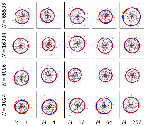
The central discovery is that the autocorrelation integral can be reliable and uncertainty-aware when estimated from the low-frequency sampling power spectrum, provided the model-fitting cutoff is selected objectively and its uncertainty is included. STACIE fits an exponential-polynomial model to the weighted low-frequency part of the periodogram, uses a two-half cross-validation criterion to identify suitable cutoffs, and marginalizes over those cutoffs to produce the final estimate and its covariance. On the ACID benchmark of 15,360 synthetic time series with known integrals, predicted uncertainties closely tracked the standard deviation of repeated estimates, error decreased with added data close to the ideal 1/sqrt(N M) scaling, and a small bias appeared only for the shortest sequences. The authors demonstrate the method on the ionic conductivity of an aqueous NaCl solution, obtaining results consistent with a prior study while reporting smaller error bars.
Load-bearing premise
The estimator assumes the input time series behave like samples of a discrete, periodic, stationary Gaussian process with zero mean, and that the true low-frequency spectrum is smooth enough to be captured by the exponential-polynomial model over the automatically selected fitting range, which may not hold exactly for real molecular dynamics currents.
Editorial extensions
If this is right
- Users can obtain transport coefficients with calibrated error bars without making subjective choices about fitting ranges, regression weights, or truncation points.
- The proposed protocol for planning the number of independent time series and checking sufficiency could become a standard workflow for equilibrium molecular dynamics simulations.
- Because the method is fully automated, it can be applied in large-scale batch analyses, making systematic benchmarking of transport-property algorithms feasible.
- The same spectral estimator applies beyond molecular dynamics to any time-correlated data, such as estimating correlation times or the uncertainty of averages in Monte Carlo and time-series analysis.
- The ACID benchmark provides a public, reproducible testbed against which future algorithms can be compared on equal footing.
Reading between the lines
- The ACID benchmark limits itself to spectra whose low-frequency part is smooth and near-quadratic, so real signals with sharp spectral features, such as pronounced resonances, may stress the automatic cutoff selection more than the published validation suggests.
- Because the method marginalizes over cutoffs rather than selecting a single one, the reported uncertainty may be conservative when the model is correct but potentially optimistic when the true spectrum lies outside the model class, a behavior that could be probed on non-Gaussian or non-smooth inputs.
- The block-averaging storage strategy implies that STACIE could be integrated into on-the-fly analysis pipelines for very long molecular dynamics runs, since only block-averaged currents need to be saved without biasing the low-frequency spectrum.
- The proposed protocol for planning simulation length could be turned into an adaptive stopping rule that extends trajectories until the sanity checks pass, which would be a natural extension for production MD workflows.
Editorial analysis
A structured set of objections, weighed in public.
Referee Report
Summary. The manuscript introduces STACIE, a spectral estimator for autocorrelation integrals from time-correlated data, with the main intended application being transport properties from equilibrium molecular dynamics simulations. The algorithm fits an exponential-polynomial model to the low-frequency sampling power spectral density, uses a smooth switching function and a cross-validation criterion (CV2L) to scan and marginalize over cutoff frequencies, and derives uncertainties from a Laplace approximation combined with cutoff averaging. The paper includes a minimal Markov-chain example, an application to the ionic conductivity of a NaCl electrolyte solution, and a large synthetic benchmark (ACID) with 15,360 cases whose autocorrelation integrals are known exactly. The authors also provide an open-source Python package, documentation, and reproducible datasets.
Significance. If the uncertainty quantification is reliable, STACIE addresses a genuine need in the molecular-dynamics community: replacing manual Green-Kubo truncation choices with a reproducible, automated procedure that also gives guidance on required simulation length. The manuscript has notable strengths: the statistical derivation of Gamma-distributed periodogram amplitudes is standard and correctly applied; the ACID benchmark is unusually large and fully reproducible; the software and data are openly available; and the electrolyte example demonstrates a realistic workflow. The central caveat is that the benchmark only tests spectra that are very close to the assumed model family, so the strong claim of reliable uncertainties for arbitrary time-correlated data is not yet fully established.
major comments (3)
- [Section 4, Eq. (17)] The ACID validation is restricted to kernels for which the first 20 discrete PSD amplitudes deviate by at most 2.5% RMS from an even quadratic, and the first 40 by at most 10%. This is essentially the model family in Eq. (17), so the benchmark is a correct-specification test. The claim that STACIE provides reliable uncertainty estimates for general time-correlated data, including EMD currents, is therefore not directly supported for spectra with strong curvature, multiple well-separated timescales, or non-analytic low-frequency behavior. I recommend adding benchmark cases with intentionally misspecified spectra (for example, sharply peaked or non-polynomial log-spectra) and reporting whether the CV2L criterion and the marginalization in Eq. (30) produce calibrated error bars in those cases.
- [Section 3.2, Table 3] The electrolyte results show substantial model dependence: the six polynomial models give conductivities from 9.92 ± 0.44 to 10.82 ± 0.27 S/m. The difference between S={0,1} and S={0,2,4} is about 0.9 S/m, which is more than three times the smallest reported standard error, and the individual error bars do not include the other model's estimate. Since the user must select the polynomial degree set and the text recommends choosing the model with the smallest predicted uncertainty, the reported per-model uncertainty does not reflect model-selection uncertainty. The paper should either automate model averaging or selection, or provide an additional uncertainty component that accounts for model choice; otherwise the 'without manual adjustment' claim is stronger than what the current evidence supports.
- [Section 2.4, Eq. (30)] The cutoff weights W_j are proportional to exp(-CV2L), where CV2L is a cross-validation proxy rather than a true likelihood. The manuscript correctly notes that the weighted likelihood cannot be used to compare cutoffs, but it does not provide a derivation or calibration argument showing that the weighted covariance in Eq. (30) remains a valid posterior covariance under model misspecification. The ACID validation only covers nearly correct models, so the calibration of the error bars under misspecification is an open question. At minimum, this should be stated as a limitation; ideally, a stress test with misspecified spectra should be added to assess whether the error bars remain reliable.
minor comments (4)
- [Section 2.7, Eq. (34)] In the block-averaging derivation, the first approximation replaces the raw signal by its block averages, which is not generally equivalent to the original spectrum. The subsequent condition B << N/k suppresses the low-frequency filtering error, but the presentation would be clearer if the error were stated as O((Bf)^2) and if the recommended block-size rule were validated numerically.
- [Supporting Information S1 and S4] There are a few typographical issues: 'OTCP' should be 'OCTP' in Table S1, and 'discription' appears in the S4 header. These are minor but should be corrected in the revised version.
- [Section 4] The statement that each kernel's PSD was 'numerically verified' to deviate by no more than 2.5% and 10% would benefit from a precise description of the verification procedure, including how the RMS deviation is computed and which frequency range is used.
- [Section 4, paragraph on limitations] The text says that the bias for short sequences is 'a known minor limitation of the current implementation of STACIE, and is a topic of ongoing research.' Since this is an admitted limitation of the algorithm's current behavior, it should also be acknowledged in the conclusions or in a dedicated limitations paragraph.
Circularity Check
No significant circularity: STACIE's estimates are validated against externally generated ground-truth data, and no predicted quantity reduces to a fitted or self-cited input.
full rationale
The core estimation chain is self-contained: the sampling PSD is computed from the input sequences, parameters are estimated by maximum a posteriori regression of the exp-poly model in Eq. (17), and the autocorrelation integral is evaluated by extrapolating the fitted model to zero frequency. Model parameters are inferred from the data rather than imposed from the known integral, and the validation compares the resulting predictions against analytically known integrals on the ACID benchmark. No equation reduces by construction to its inputs, and no fitted parameter is renamed as a prediction. The paper does contain self-citations, notably reference 19 (Toraman, Verstraelen, and Fauconnier) for the sensitivity of time-decomposition method results to regression settings, and references 61, 65, 73, 77, and 87 for the ACID dataset, the STACIE documentation, and future work. These are supporting citations or data releases, not load-bearing steps in the derivation of the estimator, and none is used to forbid alternative models or to import a uniqueness result. The ACID validation deliberately restricts the low-frequency PSDs to be close to an even quadratic, which is a coverage limitation relevant to real-spectrum misspecification and belongs in a correctness-risk assessment, not a circularity analysis. The paper's own discussion acknowledges that real MD trajectories do not fully satisfy the Gaussian and periodic assumptions, and it exposes a small bias in short-sequence cases. Overall, the derivation and validation are self-contained against external ground truth, so no significant circularity is present.
Assumptions & free parameters
free parameters (8)
- Switching steepness beta =
8 (default)
- Neff,min =
5 (default, expressed as 5P)
- gsp =
0.5 (default)
- gcv =
1.25 (default)
- gincr =
100 (default)
- Neff,max =
1000 (default)
- Polynomial degree set S =
Varies, e.g. {0,1} for electrolyte example
- Block size B for electrolyte example =
50 fs
assumptions (7)
- domain assumption Input sequences are samples of a discrete, periodic, stationary Gaussian process with zero mean.
- standard math Sampling PSD components are statistically independent and Gamma distributed with known degrees of freedom.
- domain assumption No aliasing: the MD time step is small enough that the Nyquist frequency exceeds the spectral support, and block averages faithfully represent the low-frequency PSD.
- ad hoc to paper The true low-frequency PSD is adequately described by the exponential-polynomial model in Eq. (17) over the selected cutoff range.
- ad hoc to paper The CV2L cross-validation criterion is a valid proxy for the cutoff likelihood, and a uniform prior on log cutoff is appropriate.
- standard math The Laplace approximation is accurate for the posterior distribution of model parameters.
- domain assumption Green-Kubo linear response theory relates transport properties to autocorrelation integrals.
Cite this review
Pith. "Pith review of STable AutoCorrelation Integral Estimator (STACIE): Robust and accurate transport properties from molecular dynamics simulations." pith.science (2026). https://pith.science/paper/66POMYWC
@misc{pith2026250620438,
  author       = {Pith},
  title        = {Pith review of: STable AutoCorrelation Integral Estimator (STACIE): Robust and accurate transport properties from molecular dynamics simulations},
  year         = {2026},
  howpublished = {\url{https://pith.science/paper/66POMYWC}},
  note         = {Machine review of arXiv:2506.20438}
}
read the original abstract
STACIE (STable AutoCorrelation Integral Estimator) is a novel algorithm and Python package that delivers robust, uncertainty-aware estimates of autocorrelation integrals from time-correlated data. While its primary application is deriving transport properties from equilibrium molecular dynamics simulations, STACIE is equally applicable to time-correlated data in other scientific fields. A key feature of STACIE is its ability to provide robust and accurate estimates without requiring manual adjustment of hyperparameters. Additionally, one can follow a simple protocol to prepare sufficient simulation data to achieve a desired relative error of the transport property. We demonstrate its application by estimating the ionic electrical conductivity of a NaCl-water electrolyte solution. We also present a massive synthetic benchmark dataset to rigorously validate STACIE, comprising 15360 sets of time-correlated inputs generated with diverse covariance kernels with known autocorrelation integrals. STACIE is open source and available on GitHub and PyPI, with comprehensive documentation and examples.
Figures


Figures from the paper (7 more)



Forward citations
Cited by 1 Pith paper
-
Controlling the phase behaviour of ultraconfined water via bilayer graphene stacking
AA stacking in bilayer graphene raises melting temperature of ultraconfined water by >100 K, stabilizes different ice polymorphs, and alters proton transfer relative to AB stacking via changes in the hydrogen-bond network.
Reference graph
Works this paper leans on
-
[1]
A. P. Thompson et al., “LAMMPS - a flexible simulation tool for particle-based materials modeling at the atomic, meso, and continuum scales, ” Comput. Phys. Commun., vol. 271, p. 108171, 2022, doi: 10.1016/j.cpc.2021.108171
arXiv 2022
-
[2]
S. H. Jamali et al., “OCTP: A Tool for On-the-Fly Calculation of Transport Properties of Fluids with the Order-nAlgorithm in LAMMPS, ” J. Chem. Inf. Model., vol. 59, no. 4, pp. 1290–1294, 2019, doi: 10.1021/acs.jcim.8b00939
-
[3]
Heterogeneous parallelization and acceleration of molecular dynamics simulations in GROMACS,
S. Páll et al., “Heterogeneous parallelization and acceleration of molecular dynamics simulations in GROMACS, ” J. Chem. Phys., vol. 153, no. 13, p. 134110, 2020, doi: 10.1063/5.0018516
-
[4]
Determining the shear viscosity of model liquids from molecular dynamics simulations,
B. Hess, “Determining the shear viscosity of model liquids from molecular dynamics simulations, ” J. Chem. Phys., vol. 116, no. 1, pp. 209–217, 2002, doi: 10.1063/1.1421362
-
[5]
MDAnalysis: A Python Package for the Rapid Analysis of Molecular Dynamics Simulations,
R. Gowers et al., “MDAnalysis: A Python Package for the Rapid Analysis of Molecular Dynamics Simulations, ” in Proceedings of the 15th Python in Science Conference, Austin, Texas, 2016, pp. 98–105
work page 2016
-
[6]
MDAnalysis: A toolkit for the analysis of molecular dynamics simulations,
N. Michaud‐Agrawal, E. J. Denning, T. B. Woolf, and O. Beckstein, “MDAnalysis: A toolkit for the analysis of molecular dynamics simulations, ” J. Comput. Chem., vol. 32, no. 10, pp. 2319–2327, 2011, doi: 10.1002/jcc.21787
-
[7]
tidynamics: A tiny package to compute the dynamics of stochastic and molecular simulations,
P. de Buyl, “tidynamics: A tiny package to compute the dynamics of stochastic and molecular simulations, ” J. Open Source Softw., vol. 3, no. 28, p. 877, 2018, doi: 10.21105/joss.00877
-
[8]
E. J. Baerends et al., “The Amsterdam Modeling Suite, ” J. Chem. Phys., vol. 162, no. 16, p. 162501, 2025, doi: 10.1063/5.0258496
Show all 13 references
-
[9]
QuantumATK: an integrated platform of electronic and atomic-scale modelling tools,
S. Smidstrup et al., “QuantumATK: an integrated platform of electronic and atomic-scale modelling tools, ” J. Phys.: Condens. Matter, vol. 32, no. 1, p. 15901, 2019, doi: 10.1088/1361-648x/ab4007
2019 doi
-
[10]
nMOLDYN: A program package for a neutron scattering oriented analysis of Molecular Dynamics simulations,
G. R. Kneller, V. Keiner, M. Kneller, and M. Schiller, “nMOLDYN: A program package for a neutron scattering oriented analysis of Molecular Dynamics simulations, ” Comput. Phys. Commun., vol. 91, no. 1–3, pp. 191–214, 1995, doi: 10.1016/0010-4655(95)00048-k
1995 doi
-
[11]
TRAVIS—A free analyzer for trajectories from molecular simulation,
M. Brehm, M. Thomas, S. Gehrke, and B. Kirchner, “TRAVIS—A free analyzer for trajectories from molecular simulation, ” J. Chem. Phys., vol. 152, no. 16, p. 164116410502, 2020, doi: 10.1063/5.0005078
2020 doi
-
[12]
Reliable Viscosity Calculation from Equilibrium Molecular Dynamics Simulations: A Time Decomposition Method,
Y. Zhang, A. Otani, and E. J. Maginn, “Reliable Viscosity Calculation from Equilibrium Molecular Dynamics Simulations: A Time Decomposition Method, ” J. Chem. Theory Comput., vol. 11, no. 8, pp. 3537–3546, 2015, doi: 10.1021/acs.jctc.5b00351
2015 doi
-
[13]
Accurate estimation of transport coefficients using time correlation functions without fitting any analytic forms in equilibrium simulations,
X. Liu, X. Guo, and Q. Liao, “Accurate estimation of transport coefficients using time correlation functions without fitting any analytic forms in equilibrium simulations, ” Polymer, vol. 290, p. 126519, 2024, doi: 10.1016/j.polymer.2023.126519. s45 TOC Graphic STable A utoCor...
2024
Reviewed August 6, 2026 · model on record in the stance chip above.
Discussion (0). Sign in to comment.