REVIEW 3 major objections 4 minor 65 references
A closed-form formula built from data singular values, sensor choice, and estimator predicts the double-descent spike in sparse reconstruction risk — with no free parameters.
Reviewed by Pith at T0; open to challenge. T0 means a machine referee read the full paper against a public rubric. the ladder, T0–T4 →
T0 review · deepseek-v4-flash
2026-08-01 16:28 UTC pith:6QBFB5Y2
load-bearing objection Gives an exact, data-specific risk curve for sparse-sensing double descent, and the main caveat is the unmeasured out-of-subspace test component; otherwise a solid, useful paper. the 3 major comments →
Origins and mitigation of double descent in reduced order modeling
The pith
A machine-rendered reading of the paper's core claim, the machinery that carries it, and where it could break.
Core claim
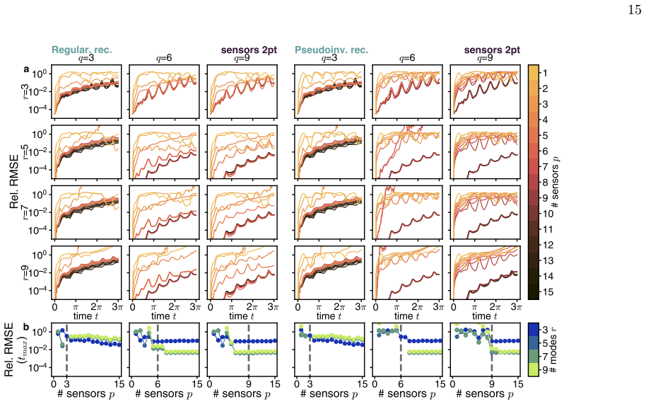
The central discovery is an explicit analytic expression, Eq. (14), for the expected reconstruction root-mean-square error of a linear sparse-sensing estimator. The expression is built from four small matrices B0..B3 that arise from the POD of the training data, the sensor selection matrix, and the estimator: B0 is the signal carried by subleading (unmodeled) modes, B1 is the error in reconstructing the leading-mode coefficients, B2 is contamination of the measured signal by subleading modes, and B3 is measurement noise. Because the cross terms are traceless, the total risk is simply the sum of squared entries of these matrices. The paper reports that this no-free-parameter formula predicts
What carries the argument
The load-bearing object is the error-covariance decomposition of Eq. (10), which rewrites the reconstruction risk as four squared B terms by treating the training-set POD covariance as the distribution of states and averaging over test states and Gaussian noise. The 'amplifier' is the matrix M that gets inverted to form the estimator: for pseudoinverse reconstruction M = ΘΘ^T for p≤r and M = Θ^TΘ for p>r, where Θ = CΨ_r is the sensing matrix of sensor rows against the leading r POD modes; for the regularized estimator M gains a diagonal prior term. When M develops very small eigenvalues, the estimator gains very large singular values and magnifies contamination or noise. The paper attributes
Load-bearing premise
The prediction treats the training-set POD covariance as the true distribution of test states and assumes every test state lies in the span of the training modes, so out-of-sample components orthogonal to the training subspace are ignored; if the test distribution drifts from the training subspace, the predicted spike height and location will be systematically wrong.
What would settle it
Run the DNA prediction on a dataset where the test set is deliberately drawn from a shifted distribution containing variance in directions orthogonal to the training POD subspace, and compare predicted vs empirical risk around p≈r: if the empirical spike appears at a different sensor count or height than predicted while contamination/noise are present, the claim of parameter-free quantitative prediction fails. A simpler check: find (or synthesize) a sensor set and r for which the Gram-matrix spectrum predicts a spike but the empirical curve is smooth — that would also falsify the amplifier mec
If this is right
- The widely used p = r sensor count is the worst operating point for unregularized reconstruction; lower p with regularization can give lower error and cost.
- Risk curves for a given dataset/sensor set can be obtained in seconds rather than tens of minutes, making thorough design-space exploration practical.
- Optimal (Bayesian ridge) regularization suppresses double descent entirely; oversampling p > r also acts as regularization by raising the small eigenvalues.
- The theory lets practitioners trace a spike to individual sensors or to correlated groups, so sensor sets can be audited and repaired rather than redesigned.
- For DEIM time integration, the parameters r, q, p should be chosen independently; operating near p ≈ q risks divergence of the reduced trajectory.
Where Pith is reading between the lines
- If the DNA formula is correct for any linear estimator, it can be turned into an optimal-experimental-design objective: minimize the predicted peak risk directly rather than relying on greedy placement; the paper gestures at this but does not develop the optimization.
- The orthogonality-crisis argument implies a fundamental trade-off for any linear reconstruction with fewer sensors than modes: regularize or accept a spike somewhere near p≈r; this should hold for any orthonormal basis, not just POD, and could be tested with synthetic random orthogonal bases.
- The full error covariance, not just its trace, could produce calibrated per-pixel uncertainty maps for safety-critical reconstructions; the paper notes the earlier heatmap was under-calibrated because it was noise-only but does not test whether the four-term covariance fixes calibration.
- The theory's reliance on the training POD covariance as the test distribution suggests an immediate testable extension: shift the test distribution (e.g., climate-change-like drift in SST) and measure how the predicted spike degrades; this quantifies how far the no-free-parameter claim extends out of distribution.
Editorial analysis
A structured set of objections, weighed in public.
Referee Report
Summary. This paper develops a Data-Noise Averaging (DNA) theory for the reconstruction risk of sparse-sensing/reduced-order models. Under the model x = Ψ_r a_r + Ψ_c a_c, with sensors y = Cx + Δy and a linear estimator â_r = A y, the authors derive a covariance decomposition of the reconstruction error (Eq. 10) into contributions from subleading modes, leading-mode reconstruction error, contamination, and noise. This yields a closed-form RMSE expression (Eq. 14) computed from the training POD singular values, the sensor selection matrix, and the estimator A, with no fitted parameters. The theory is applied to static SST reconstruction for 16 design combinations and to DEIM/NSE nonlinear-term reconstruction and time integration. The authors show that double-descent spikes coincide with the appearance of low-lying eigenvalues of the inversion matrix M, distinguish 1-point vs ensemble sensor failures, and demonstrate regularization and undersampling as mitigations. They report a ~10^3 computational speedup over empirical risk averaging.
Significance. The paper's central contribution is a closed-form, parameter-free prediction of reconstruction risk that does not rely on random-matrix universality. If it holds for out-of-sample states, it is a practically valuable tool for sensor placement and ROM design: risk curves and double-descent spikes can be computed in seconds rather than by repeated empirical evaluation. The derivation is algebraically correct under the stated model, and the SST validation across all 16 binary factor combinations, including the location and magnitude of the spike and the minute localized jumps, is impressive. The spectral analysis tying the spike to low-lying eigenvalues of M and the distinction between 1-point and ensemble failures is insightful. The computational complexity analysis is transparent and the claimed speedup is plausible.
major comments (3)
- [III.A, Eq. (7)] The derivation replaces the test-state covariance with the training sample covariance (Eq. 7) and represents states through Ψ_r and Ψ_c only (Eq. 1). For held-out states with components orthogonal to span(X_train), the term E[P⊥ x x^T P⊥] is missing from K (Eq. 10). The full-state SST panels in Fig. 4 show agreement with test risk, but the paper never quantifies this residual. If it is non-negligible (e.g., under distribution shift), Eq. (14) will systematically underestimate test risk. Please either add this term, or measure and bound the out-of-subspace variance for the SST test set, and revise the 'any setup' claim in §VI.A accordingly.
- [V.C, Fig. 9] The DEIM static nonlinearity reconstruction is validated on the same snapshots used to build the POD basis: the paper states 'we do not separate the data into train and test sets as they would be identical' (§V.C). The empirical curves in Fig. 9 are therefore in-sample; the agreement with DNA is expected because DNA computes risk under the training covariance. This does not validate the theory for unseen states in the DEIM setting. The time-integration experiments (Fig. 10) are more informative, but the static validation should be re-run on a held-out portion of the trajectory (e.g., one of the six periods) or the in-sample nature should be explicitly flagged as a limitation.
- [VI.A] The Discussion states that DNA provides 'a computationally cheap yet accurate approximation of the reconstruction error covariance matrix for any linear reconstruction setup and any sensor set.' This universality claim is not supported by the derivation, which assumes test states lie in the training POD subspace. As written, the theory is exact for states in span(X_train); the empirical support for out-of-subspace states is indirect. Please qualify this claim to match the evidence, or provide additional experiments with a distribution shift.
minor comments (4)
- [Eq. (14)] The notation in Eq. (14) could be clarified: the elementwise squaring of the B_l matrices and the summation over their differing index ranges is described in the text, but a reader may initially misread the formula as a matrix product. A brief explicit example or a sentence defining the elementwise square would help.
- [Fig. 3] The purple and brown shaded areas representing test and train means overlap almost everywhere, making the two distributions hard to distinguish. Consider plotting the test and train curves with different line styles or in separate panels for the key configurations.
- [IV.D] The sentence 'addition of of a positive diagonal contribution' contains a duplicated 'of'.
- [Eq. (28)] The definition of η²_reg is ambiguous: 'max X_{i=q+1} σ²_i' could be read as a maximum or a sum. Please clarify the intended expression (e.g., a sum over subleading singular values or the largest subleading singular value).
Circularity Check
The central DNA prediction is independently tested on held-out SST data; only the NSE/DEIM static validation is in-sample, which is a minor circularity.
specific steps
-
other
[Sec. V C, 'Reconstructing the nonlinear term' (paragraph after Eq. 30)]
"In addition, since the ground truth data is periodic (up to the integration error of the full-order model), we do not separate the data into train and test sets as they would be identical."
In the NSE/DEIM static reconstruction study, the same periodic snapshots are used both to build the POD basis and to compute the empirical RMSE curves in Fig. 9. The DNA prediction uses exactly the training covariance of those snapshots (Eq. 7), so the predicted and empirical curves are expected to coincide by construction, up to finite-sample noise and the N vs. N-1 normalization. Thus the Fig. 9 match is a self-consistency check rather than an out-of-sample prediction. This does not affect the main SST claim, where a separate 20% test set is held out, but it is a genuine in-sample validation for the DEIM static case.
full rationale
The core DNA derivation is self-contained: Eq. (10) and Eq. (14) follow algebraically from the stated linear reconstruction model, the POD decomposition, and the training-set covariance assumption (Eq. 7). No parameter is fitted to the empirical risk curves, and the prediction for the SST case study is validated on a held-out 20% test set, so the central double-descent prediction has independent empirical content. The regularized estimator and sensor-placement algorithm are cited from the authors' prior work, but these citations are not load-bearing for the circularity question: the estimator is a standard ridge/MAP formula and the algorithm's role is to generate a sensor ordering, not to enforce the predicted risk curve. The only notable circularity is explicitly acknowledged by the authors in the NSE/DEIM static reconstruction, where train and test sets are not separated because the data are periodic. There, the DNA prediction is effectively an analytic evaluation of the training-set error, so the agreement in Fig. 9 is by construction to a large degree. This is a minor, localized circularity, not one that undermines the paper's central claim.
Axiom & Free-Parameter Ledger
free parameters (5)
- Number of retained modes r (SST) / q (NSE) =
r=100 for SST; q=3,6,9 for NSE
- Noise level η_noise (SST noisy scenarios) =
0.5 σ_scale
- Regularization strength η_reg (regularized reconstruction) =
SST: equal to η_noise=0.5σ_scale; NSE: computed from Eq. 28 (subleading singular values)
- Sensor budget p_max =
200 for SST, 40 for NSE
- Regularization scaling Q (Fig. 7 sweep) =
swept around 1
axioms (6)
- domain assumption Test states lie in the span of the training POD modes (x = Ψr a_r + Ψc a_c).
- domain assumption The empirical training covariance equals the true data covariance.
- domain assumption Measurement noise is Gaussian, uncorrelated, with covariance η² I_p, and independent of the state.
- domain assumption The reconstruction matrix A is always full rank (rank = min(r,p)).
- ad hoc to paper For NSE/DEIM, the state-approximation error acts as an effective noise with covariance assigned by Eq. (28).
- domain assumption No set of r sensing vectors from the n candidate locations can be made orthogonal.
read the original abstract
Latent low-dimensional structure in datasets of natural and engineered systems enables their sparse sensing, or full-state reconstruction from historical data and very few carefully chosen localized measurements. Depending on the reconstruction algorithm, sensor locations, and measurement noise, the reconstruction risk curves demonstrate a diversity of patterns including a dramatic peak in error known as double descent in Machine Learning literature. Here we explore those scenarios under a unified Data-Noise Averaging theory. Qualitatively, we formulate sufficient criteria for double descent to emerge through a catastrophic amplification of a pathological signal in reconstruction. Quantitatively, we predict the detailed risk curves at a fraction of computational cost, trace reconstruction instability to individual sensors and their combinations, and provide regularization mechanisms to mitigate the instability. We demonstrate results for both static reconstruction of Sea Surface Temperature patterns and time integration of a reduced order model of a PDE.
Figures



Reference graph
Works this paper leans on
-
[1]
measurements
DEIM modes and reconstruction The tailored modes for the state itself and the nonlin- ear reconstruction are found by two separate PODs: X=UΣV ⊤ ≈U rΣrV⊤ r (24) XN L=ΞΣN LVN L,⊤≈Ξ qΣN L q VN L,⊤ q ,(25) where the subscriptsr, qdenote truncation to the spec- ified number of modes. Since sparse sensing is only ap- plied to the nonlinear term, we only need t...
-
[2]
p-inv.”) and regularized (“reg
Complex-valued corrections Additional care in DEIM construction needs to be taken to account for complex-valued fields used in some PDEs. If the stateuis complex valued, so are usually the state and nonlinearity data matricesX,X N L. POD can still be straightforwardly computed for a complex- valued matrix. The resulting singularvaluesare real, as the comp...
-
[3]
D. J. Lucia, P. S. Beran, and W. A. Silva, Reduced-order modeling: new approaches for computational physics, Progress in aerospace sciences40, 51 (2004)
2004
-
[4]
J. Yu, C. Yan, and M. Guo, Non-intrusive reduced-order modeling for fluid problems: A brief review, Proceedings of the Institution of Mechanical Engineers, Part G: Jour- nal of Aerospace Engineering233, 5896 (2019)
2019
-
[5]
J. N. Kutz, Machine learning methods for reduced order modeling, inModel Order Reduction and Applications: Cetraro, Italy 2021(Springer, 2023) pp. 201–228
2021
-
[6]
Manohar, B
K. Manohar, B. W. Brunton, J. N. Kutz, and S. L. Brun- ton, Data-driven sparse sensor placement for reconstruc- tion: Demonstrating the benefits of exploiting known patterns, IEEE Control Systems Magazine38, 63 (2018)
2018
-
[7]
Barrault, Y
M. Barrault, Y. Maday, N. C. Nguyen, and A. T. Pat- era, An ‘empirical interpolation’method: application to efficient reduced-basis discretization of partial differen- tial equations, Comptes Rendus Mathematique339, 667 (2004)
2004
-
[8]
Chaturantabut and D
S. Chaturantabut and D. C. Sorensen, Discrete empirical interpolation for nonlinear model reduction, inProceed- ings of the 48h IEEE Conference on Decision and Con- trol (CDC) held jointly with 2009 28th Chinese Control Conference(IEEE, 2009) pp. 4316–4321
2009
-
[9]
Drmac and S
Z. Drmac and S. Gugercin, A new selection operator for the discrete empirical interpolation method—improved a priori error bound and extensions, SIAM Journal on Scientific Computing38, A631 (2016)
2016
-
[10]
Kakasenko, A
L. Kakasenko, A. Alexanderian, M. Farazmand, and A. K. Saibaba, Bridging the gap between deterministic and probabilistic approaches to state estimation, Physica D: Nonlinear Phenomena (2026)
2026
-
[11]
N. Karnik, C. Wang, P. K. Bhowmik, J. J. Cogliati, S. A. Balderrama Prieto, C. Xing, A. A. Klishin, R. Skifton, M. Moussaoui, C. P. Folsom, J. J. Palmer, P. Sabharwall, K. Manohar, and M. G. Abdo, Leveraging optimal sparse sensor placement to aggregate a network of digital twins for nuclear subsystems, Energies17, 10.3390/en17133355 (2024)
-
[12]
Farazmand, Sparse discrete empirical interpolation method: State estimation from few sensors, SIAM Jour- nal on Scientific Computing46, A3658 (2024)
M. Farazmand, Sparse discrete empirical interpolation method: State estimation from few sensors, SIAM Jour- nal on Scientific Computing46, A3658 (2024)
2024
-
[13]
Farazmand, State estimation using sparse deim and recurrent neural networks, Proceedings of the Royal Soci- ety A: Mathematical, Physical and Engineering Sciences 482(2026)
M. Farazmand, State estimation using sparse deim and recurrent neural networks, Proceedings of the Royal Soci- ety A: Mathematical, Physical and Engineering Sciences 482(2026)
2026
-
[14]
Everson and L
R. Everson and L. Sirovich, Karhunen–loeve procedure for gappy data, JOSA A12, 1657 (1995)
1995
-
[15]
Yildirim, C
B. Yildirim, C. Chryssostomidis, and G. Karniadakis, Efficient sensor placement for ocean measurements us- ing low-dimensional concepts, Ocean Modelling27, 160 (2009)
2009
-
[16]
Willcox, Unsteady flow sensing and estimation via the gappy proper orthogonal decomposition, Computers & fluids35, 208 (2006)
K. Willcox, Unsteady flow sensing and estimation via the gappy proper orthogonal decomposition, Computers & fluids35, 208 (2006)
2006
-
[17]
A. A. Klishin, J. N. Kutz, and K. Manohar, Data-induced interactions of sparse sensors using statistical physics, arXiv preprint arXiv:2307.11838 (2023)
arXiv 2023
-
[18]
M. Loog, T. Viering, and A. Mey, Minimizers of the em- pirical risk and risk monotonicity, Advances in Neural Information Processing Systems32(2019)
2019
-
[19]
Viering and M
T. Viering and M. Loog, The shape of learning curves: a review, IEEE Transactions on Pattern Analysis and Machine Intelligence45, 7799 (2022)
2022
-
[20]
Clark, S
E. Clark, S. L. Brunton, and J. N. Kutz, Multi-fidelity sensor selection: Greedy algorithms to place cheap and expensive sensors with cost constraints, IEEE Sensors Journal21, 600 (2020)
2020
-
[21]
B. M. de Silva, K. Manohar, E. Clark, B. W. Brunton, S. L. Brunton, and J. N. Kutz, Pysensors: A python package for sparse sensor placement, arXiv preprint arXiv:2102.13476 (2021)
Pith/arXiv arXiv 2021
-
[22]
de Silva, K
B. de Silva, K. Manohar, and E. Clark, Py- Sensors Examples / Basis comparison,https: //python-sensors.readthedocs.io/en/latest/ examples/basis_comparison.html(2020), accessed: 2026-07-21
2020
-
[23]
Belkin, D
M. Belkin, D. Hsu, S. Ma, and S. Mandal, Reconciling modern machine-learning practice and the classical bias– variance trade-off, Proceedings of the National Academy of Sciences116, 15849 (2019)
2019
-
[24]
Nakkiran, G
P. Nakkiran, G. Kaplun, Y. Bansal, T. Yang, B. Barak, and I. Sutskever, Deep double descent: Where bigger models and more data hurt, Journal of Statistical Me- chanics: Theory and Experiment2021, 124003 (2021)
2021
-
[25]
Breiman and D
L. Breiman and D. Freedman, How many variables should be entered in a regression equation?, Journal of the Amer- ican Statistical Association78, 131 (1983)
1983
-
[26]
Vallet, J.-G
F. Vallet, J.-G. Cailton, and P. Refregier, Linear and non- linear extension of the pseudo-inverse solution for learn- 19 ing boolean functions, EPL (Europhysics Letters)9, 315 (1989)
1989
-
[27]
Opper, W
M. Opper, W. Kinzel, J. Kleinz, and R. Nehl, On the ability of the optimal perceptron to generalise, Journal of Physics A: Mathematical and General23, L581 (1990)
1990
-
[28]
T. L. Watkin, A. Rau, and M. Biehl, The statistical me- chanics of learning a rule, Reviews of Modern Physics65, 499 (1993)
1993
-
[29]
Raudys and R
S. Raudys and R. P. Duin, Expected classification error of the fisher linear classifier with pseudo-inverse covariance matrix, Pattern recognition letters19, 385 (1998)
1998
-
[30]
R. P. Duin, Classifiers in almost empty spaces, inPro- ceedings 15th International Conference on Pattern Recog- nition. ICPR-2000, Vol. 2 (IEEE, 2000) pp. 1–7
2000
-
[31]
M. Loog, T. Viering, A. Mey, J. H. Krijthe, and D. M. Tax, A brief prehistory of double descent, Proceedings of the National Academy of Sciences117, 10625 (2020)
2020
-
[32]
d’Ascoli, L
S. d’Ascoli, L. Sagun, and G. Biroli, Triple descent and the two kinds of overfitting: Where & why do they ap- pear?, Advances in neural information processing sys- tems33, 3058 (2020)
2020
-
[33]
M. K. Transtrum, G. L. Hart, T. J. Jarvis, and J. P. Whitehead, Generalized aliasing explains double descent and informs model design, Physical Review Research7, 043268 (2025)
2025
-
[34]
Nakkiran, P
P. Nakkiran, P. Venkat, S. M. Kakade, and T. Ma, Opti- mal regularization can mitigate double descent, inInter- national Conference on Learning Representations(2021)
2021
-
[35]
J. H. Krijthe and M. Loog, The peaking phenomenon in semi-supervised learning, inJoint IAPR International Workshops on Statistical Techniques in Pattern Recogni- tion (SPR) and Structural and Syntactic Pattern Recog- nition (SSPR)(Springer, 2016) pp. 299–309
2016
-
[36]
d’Ascoli, M
S. d’Ascoli, M. Refinetti, G. Biroli, and F. Krzakala, Dou- ble trouble in double descent: Bias and variance(s) in the lazy regime, inInternational Conference on Machine Learning(PMLR, 2020) pp. 2280–2290
2020
-
[37]
Belkin, D
M. Belkin, D. Hsu, and J. Xu, Two models of double descent for weak features, SIAM Journal on Mathematics of Data Science2, 1167 (2020)
2020
-
[38]
Hastie, A
T. Hastie, A. Montanari, S. Rosset, and R. J. Tibshirani, Surprises in high-dimensional ridgeless least squares in- terpolation, Annals of statistics50, 949 (2022)
2022
-
[39]
Mei and A
S. Mei and A. Montanari, The generalization error of random features regression: Precise asymptotics and the double descent curve, Communications on Pure and Ap- plied Mathematics75, 667 (2022)
2022
-
[40]
Spigler, M
S. Spigler, M. Geiger, S. d’Ascoli, L. Sagun, G. Biroli, and M. Wyart, A jamming transition from under-to over- parametrization affects generalization in deep learning, Journal of Physics A: Mathematical and Theoretical52, 474001 (2019)
2019
-
[41]
J. W. Rocks and P. Mehta, Memorizing without overfit- ting: Bias, variance, and interpolation in overparameter- ized models, Physical review research4, 013201 (2022)
2022
- [42]
-
[43]
Gedon, A
D. Gedon, A. H. Ribeiro, and T. B. Sch¨ on, No dou- ble descent in principal component regression: A high- dimensional analysis, inProceedings of the 41st In- ternational Conference on Machine Learning, Proceed- ings of Machine Learning Research, Vol. 235, edited by R. Salakhutdinov, Z. Kolter, K. Heller, A. Weller, N. Oliver, J. Scarlett, and F. Berkenka...
2024
-
[44]
Gavish and D
M. Gavish and D. L. Donoho, The optimal hard thresh- old for singular values is 4/ √ 3, IEEE Transactions on Information Theory60, 5040 (2014)
2014
-
[45]
Udell and A
M. Udell and A. Townsend, Why are big data matrices approximately low rank?, SIAM Journal on Mathematics of Data Science1, 144 (2019)
2019
-
[46]
K. N. Quinn, M. C. Abbott, M. K. Transtrum, B. B. Machta, and J. P. Sethna, Information geometry for mul- tiparameter models: New perspectives on the origin of simplicity, Reports on Progress in Physics (2022)
2022
- [47]
-
[48]
Huang, C
B. Huang, C. Liu, V. Banzon, E. Freeman, G. Graham, B. Hankins, T. Smith, and H.-M. Zhang, Improvements of the daily optimum interpolation sea surface tempera- ture (DOISST) version 2.1, Journal of Climate34, 2923 (2021)
2021
-
[49]
J. R. Bunch and C. P. Nielsen, Updating the singular value decomposition, Numerische Mathematik31, 111 (1978)
1978
-
[50]
J. H. Wilkinson,The algebraic eigenvalue problem, Vol. 662 (Clarendon, Oxford, 1965)
1965
-
[51]
R. C. Thompson, The behavior of eigenvalues and singu- lar values under perturbations of restricted rank, Linear Algebra and its Applications13, 69 (1976)
1976
-
[52]
F. R. Gantmacher and M. G. Krein,Oscillation matri- ces and kernels and small vibrations of mechanical sys- tems: revised edition(AMS Chelsea Publishing, Provi- dence, RI, 2002)
2002
-
[53]
S. L. Brunton and J. N. Kutz,Data-driven science and engineering: Machine learning, dynamical systems, and control, 2nd ed. (Cambridge University Press, 2022)
2022
-
[54]
A. A. Klishin and D. S. Bassett, Exposure theory for learning complex networks with random walks, Journal of Complex Networks10, cnac029 (2022)
2022
-
[55]
A. A. Klishin, N. H. Christianson, C. S. Siew, and D. S. Bassett, Learning dynamic graphs, too slow, arXiv preprint arXiv:2207.02177 (2022)
Pith/arXiv arXiv 2022
-
[56]
Peherstorfer, Z
B. Peherstorfer, Z. Drmac, and S. Gugercin, Stability of discrete empirical interpolation and gappy proper orthog- onal decomposition with randomized and deterministic sampling points, SIAM Journal on Scientific Computing 42, A2837 (2020)
2020
-
[57]
J. P. Williams, O. Zahn, and J. N. Kutz, Sensing with shallow recurrent decoder networks, Proceedings of the Royal Society A: Mathematical, Physical and Engineer- ing Sciences480(2024)
2024
-
[58]
Tomasetto, J
M. Tomasetto, J. P. Williams, F. Braghin, A. Manzoni, and J. N. Kutz, Reduced order modeling with shallow recurrent decoder networks, Nature Communications16, 10260 (2025)
2025
-
[59]
Chaloner and I
K. Chaloner and I. Verdinelli, Bayesian experimental de- sign: A review, Statistical science , 273 (1995)
1995
-
[60]
E. G. Ryan, C. C. Drovandi, J. M. McGree, and A. N. Pettitt, A review of modern computational algorithms for Bayesian optimal design, International Statistical Review 84, 128 (2016)
2016
-
[61]
Alexanderian, Optimal experimental design for infinite-dimensional Bayesian inverse problems governed 20 by pdes: A review, Inverse Problems37, 043001 (2021)
A. Alexanderian, Optimal experimental design for infinite-dimensional Bayesian inverse problems governed 20 by pdes: A review, Inverse Problems37, 043001 (2021)
2021
-
[62]
Rainforth, A
T. Rainforth, A. Foster, D. R. Ivanova, and F. Bick- ford Smith, Modern Bayesian experimental design, Sta- tistical Science39, 100 (2024)
2024
-
[63]
Karnik, M
N. Karnik, M. G. Abdo, C. E. Estrada-Perez, J. S. Yoo, J. J. Cogliati, R. S. Skifton, P. Calderoni, S. L. Brun- ton, and K. Manohar, Constrained optimization of sensor placement for nuclear digital twins, IEEE Sensors Jour- nal , 1 (2024)
2024
-
[64]
Crameri, Scientific colour maps (2023)
F. Crameri, Scientific colour maps (2023)
2023
-
[65]
C. S. Adorf, P. M. Dodd, V. Ramasubramani, and S. C. Glotzer, Simple data and workflow management with the signac framework, Computational Materials Science146, 220 (2018)
2018
discussion (0)
Sign in with ORCID, Apple, or X to comment. Anyone can read and Pith papers without signing in.