REVIEW 4 major objections 5 minor 1 cited by
This paper argues that a shallow quantum neural network, trained on real daily weather data, can match or beat a classical recurrent baseline in short- and medium-term forecasting, with the strongest edge in wind speed.
Reviewed by Pith at T0; open to challenge. T0 means a machine referee read the full paper against a public rubric. the ladder, T0–T4 →
T0 review · deepseek-v4-flash
2026-08-05 12:33 UTC pith:7IU6BD3W
load-bearing objection A small but honest QML weather-forecasting study whose central comparison is plausible but not yet established; the missing feature-date alignment is the thing that needs fixing. the 4 major comments →
Exploring Quantum Machine Learning for Weather Forecasting
The pith
A machine-rendered reading of the paper's core claim, the machinery that carries it, and where it could break.
Core claim
On the paper's own terms, the central discovery is that a low-depth variational quantum circuit can be trained on real meteorological data to forecast temperature and wind speed with accuracy on par with—and in the best configurations better than—a classical recurrent baseline. The quantum model's forecast distributions sit closer to observed values on days with sharp weather changes, which the authors attribute to the QNN's ability to capture nonlinear patterns without long-range memory. They also find that network depth and entanglement strategy affect performance nonlinearly, so the best configuration differs between temperature and wind speed.
What carries the argument
The load-bearing object is a parameterized quantum circuit: each selected climate feature is encoded as a Ry rotation on one qubit, the qubits are entangled with either a simple entangling layer or a strongly entangling layer, and trainable rotation angles are updated by a classical optimizer after projective measurement. The paper varies only the number of variational layers (1, 3, or 5) and the entanglement strategy, holding data, optimizer, and training budget fixed, which isolates the architectural effect on forecasting skill.
Load-bearing premise
The load-bearing premise is that every input feature is known before the forecast horizon starts; if humidity, solar irradiance, or a lagged variable is measured on the target day, the reported mean absolute errors are not genuine forecasts.
What would settle it
Look at the timestamps of the six (temperature) or eight (wind) features used for the test days in the POWER data. If any feature value falls on or after the first forecast day, re-run the comparison with features shifted so all inputs predate the horizon; the claimed QNN edge would disappear if those same-day features carried the signal.
If this is right
- If the reported results hold, quantum neural networks deserve inclusion in short- and medium-term regression benchmarks, not just classification tasks.
- The QNN's better handling of abrupt temperature and wind shifts suggests quantum models could be tested for extreme-event forecasting, the regime where classical models are weakest.
- Because shallow circuits matched or beat deeper ones, future quantum forecasting work should focus on circuit structure rather than brute-force depth.
- The faster convergence observed for temperature suggests QNNs may be a practical choice when training budgets are tight.
Where Pith is reading between the lines
- The comparison is only meaningful if every input feature is known before the forecast window begins; the paper never states this temporal alignment, so the reported edge over the RNN is conditional on that unstated assumption.
- A natural extension is a strict forecast test where features are shifted backward by the full horizon, so no same-day information leaks into the predictors; this would tell whether the QNN advantage survives a true out-of-sample forecast.
- The same architecture could be stress-tested on multi-year data from other climates, where abrupt shifts are more frequent, to see whether the adaptability claim generalizes.
- Because the test sets are tiny (14 and 5 days), the MAE differences lie within plausible sampling noise; a larger test window is needed to confirm the quantum edge.
Editorial analysis
A structured set of objections, weighed in public.
Referee Report
Summary. The paper reports a proof-of-concept comparison between a variational Quantum Neural Network (QNN) and a classical Recurrent Neural Network (RNN) for short/medium-term weather forecasting at a single Brazilian location, using one year of daily NASA POWER data. Six QNN configurations (two entanglement strategies, three depths) are compared against an RNN baseline for 14-day temperature and 5-day wind-speed forecasting. The reported test-set MAEs favor the best QNN configuration (0.304 vs 0.357 for temperature, 0.156 vs 0.167 for wind speed), and the authors further claim qualitative advantages in adaptability to abrupt shifts and in training speed for temperature. The manuscript includes reproducibility information and cites a public code repository.
Significance. If the central claim were established, the paper would provide evidence that small variational QNNs can be competitive with classical recurrent models on structured meteorological time series, and it would add a useful data point to the sparse literature on QML for regression. The authors deserve credit for using real meteorological data, for running 10 repetitions per configuration, for reporting training/validation loss curves, and for making source code available in a public repository (reference [42]). However, the quantitative evidence is currently not strong enough: the test sets contain only 14 and 5 points, the best configuration is selected on the same test set with no multiplicity correction or uncertainty interval, the classical baseline is trained with different hyperparameters and much longer epoch counts, and the temporal alignment of input features to forecast targets is not specified. These issues are load-bearing because the gap to the RNN is small and could be explained by leakage, tuning artifacts, or noise. With the requested clarifications and a more careful statistical analysis, the result would be a solid, if modest, contribution; in its present form it is an
major comments (4)
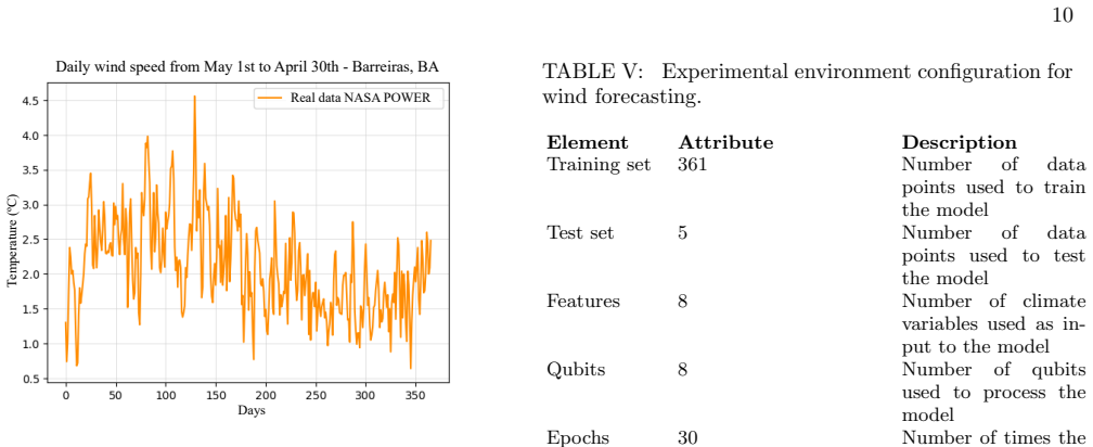
- [II B, III A, III B, Tables III and V] The paper never states the temporal alignment of the input features to the forecast targets. Section II B only says that lags of 28 days (temperature) and 6 days (wind speed) were appended; it does not say whether the five or seven climate variables (humidity, solar irradiance, etc.) are values from the forecast origin, from the target date, or from some other date. Tables III and V list only the number of features, not their dates relative to the horizon. Since the test horizon is 14 or 5 days, any feature observed inside that window would make the reported MAEs nowcasts rather than forecasts and would invalidate the comparison. Please specify precisely, for each sample, which calendar dates are used for each input feature and which date is the forecast target, and confirm that all inputs are known before the forecast window begins. The code in repository [42] should make this explicit.
- [II C, III A 2, III B 2] The central quantitative claim rests on test MAEs computed on 14 and 5 test points. No uncertainty intervals are reported for the MAE values; Table IV and Table VI give only point estimates for each configuration, despite the paper stating that 10 runs were performed. With test sizes this small, the differences (0.304 vs 0.357 and 0.156 vs 0.167) may be within run-to-run and sampling variability. In addition, the best QNN configuration is selected after inspecting the same test set on which it is then reported, which introduces selection bias and inflates the apparent advantage. Please report the distribution of the 10 per-run MAEs, provide standard errors or confidence intervals, and, if the best configuration is chosen from the six, account for the multiple comparisons (e.g., by reporting all configurations and applying a simple correction, or by using a validation split for model sele
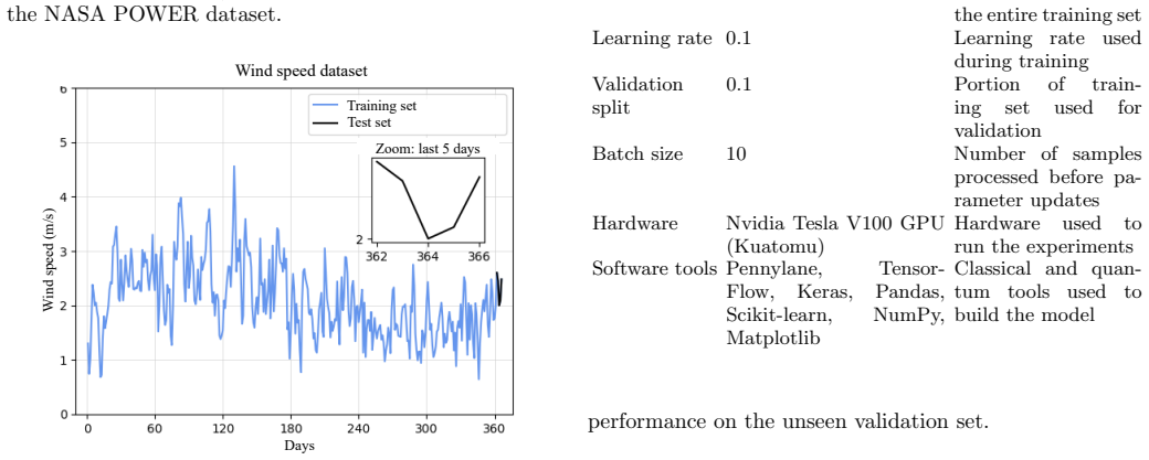
- [II A, III A, III B] The comparison between QNN and RNN is not controlled: the QNN uses learning rate 0.1 and 30 epochs, while the RNN uses learning rate 0.001 and 500 epochs (Tables III and V and the text in Sections III A 2 and III B 2). The RNN also uses 256 neurons, whereas the QNN uses 6 or 8 qubits. Differences in optimization budget and model capacity are confounded with the quantum/classical distinction. At minimum, the authors should either tune the RNN to a similar practical training budget, provide a sensitivity analysis of the RNN to learning rate and epoch count, or explicitly state that the comparison is between one particular QNN implementation and one particular RNN implementation, and temper the abstract's language accordingly.
- [II B, III A, III B] The evaluation uses a single train/test split at the end of a one-year series, with no seasonal coverage (10 days for temperature, 5 days for wind). This design is particularly fragile for weather data, which is strongly seasonal and autocorrelated. The claim of 'abrupt data shift' adaptability is based on a single day (day 11 in temperature, day 1 in wind) in each split. Please add rolling-origin evaluation or at least multiple test windows, and avoid drawing general conclusions about 'abrupt shifts' from one or two points.
minor comments (5)
- [Section III A 2] The text says 'the MAE of 0.347 achieved by the RNN' immediately after presenting Table IV, which reports 0.357. Please correct the inconsistency.
- [Figures 9-12, 20] Several figure cross-references in Section III are mislabeled: the classical temperature mean prediction is referred to as 'Figure 19' instead of Figure 11, and the classical wind loss is referred to as 'Figure 20' instead of Figure 12/20 depending on section. Figure 14's caption says 'daily temperature data' but the panel shows wind speed. Please renumber and cross-check all figure references.
- [Figure 5] The caption refers to 'the presented INN' where it presumably means 'QNN' or 'VQA'. Please fix the typo.
- [Eq. (1), Tables IV and VI] The data are standardized with Eq. (1), so the reported MAE values are in standardized units, not in °C or m/s. The manuscript does not state this, which makes the numbers hard to interpret. Please clarify in the metric definitions or in the table captions.
- [Reference [42]] The repository reference is incomplete: it says 'gitHub repository' without a URL or identifier. A complete link is needed to support the reproducibility claim.
Circularity Check
No circular reduction; only minor self-citation for QNN architecture, not load-bearing.
full rationale
The paper's claimed derivation is an empirical benchmark: a QNN architecture (encoding six/eight features, parameterized rotations, measured and classically optimized) is trained on NASA POWER data and compared to an RNN under matched train/test splits; the reported MAEs (0.304 vs 0.357 for temperature, 0.156 vs 0.167 for wind) are computed on held-out terminal segments and are not algebraic functions of the training inputs or of the fitted parameters. The only self-citation is the architectural lineage: 'designed following the approach proposed by Oğur [38] and further explored by Jesus [39]' (Sec. II C 1), where [39] shares authors with this paper. That citation supplies the ansatz (Ry encoding + variational layers + entanglement strategy), but it does not by itself determine the comparative result; the same architecture could have lost, and the empirical outcomes are externally grounded in the dataset. I therefore identify no circular step: no quantity called a prediction is identical by construction to a fitted input, no uniqueness theorem is imported from the authors' prior work, and no known result is merely renamed. The unspecified temporal alignment of features is a validity risk (if covariates come from inside the forecast window, the experiment is nowcasting), but that would be data leakage, not circularity; it does not affect this score.
Axiom & Free-Parameter Ledger
free parameters (5)
- Lag periods =
28 days (temperature), 6 days (wind)
- Feature correlation threshold =
|rho| >= 0.3
- QNN hyperparameters =
lr=0.1, 30 epochs, batch size 10
- Best architecture selection =
Exp 2, 1 layer (temp); Exp 1, 3 layers (wind)
- Validation split and seeds =
0.1 split; seeds not reported
axioms (4)
- domain assumption NASA POWER daily weather data for Barreiras is an adequate ground-truth source
- domain assumption Pearson correlation is a valid guide to predictive features and lags for a nonlinear model
- ad hoc to paper The variational QNN architecture of Oğur [38] and Jesus [39] is appropriate for time-series regression
- ad hoc to paper Input features are observed before the forecast horizon (no data leakage)
Cite this review
Pith. "Pith review of Exploring Quantum Machine Learning for Weather Forecasting." pith.science (2026). https://pith.science/paper/7IU6BD3W
@misc{pith2026250901422,
  author       = {Pith},
  title        = {Pith review of: Exploring Quantum Machine Learning for Weather Forecasting},
  year         = {2026},
  howpublished = {\url{https://pith.science/paper/7IU6BD3W}},
  note         = {Machine review of arXiv:2509.01422}
}
read the original abstract
Weather forecasting plays a crucial role in supporting strategic decisions across various sectors, including agriculture, renewable energy production, and disaster management. However, the inherently dynamic and chaotic behavior of the atmosphere presents significant challenges to conventional predictive models. On the other hand, introducing quantum computing simulation techniques to the forecasting problems constitutes a promising alternative to overcome these challenges. In this context, this work explores the emerging intersection between quantum machine learning (QML) and climate forecasting. We present the implementation of a Quantum Neural Network (QNN) trained on real meteorological data from NASA's Prediction of Worldwide Energy Resources (POWER) database. The results show that QNN has the potential to outperform a classical Recurrent Neural Network (RNN) in terms of accuracy and adaptability to abrupt data shifts, particularly in wind speed prediction. Despite observed nonlinearities and architectural sensitivities, the QNN demonstrated robustness in handling temporal variability and faster convergence in temperature prediction. These findings highlight the potential of quantum models in short and medium term climate prediction, while also revealing key challenges and future directions for optimization and broader applicability.
Figures




Forward citations
Cited by 1 Pith paper
-
How Hard Is Quantum Advantage? A Cloud Microphysics Stress Test for Variational Quantum Models
Even after rich frequency encoding, classical post-processing, and extensive hyperparameter search, hybrid QNNs underperform simple FCNNs on cloud microphysics parameterization.
Reference graph
Works this paper leans on
-
[1]
Quantum Neural Network (QNN) The quantum predictive model employed in this study is a Quantum Neural Network (QNN), designed following the approach proposed by O˘ gur [38] and further explored by Jesus [39] in demand forecasting for the financial sec- tor. The operating principle of the underlying variational quantum algorithm—where classical features xi ...
-
[2]
Recurrent Neural Network (RNN) The classical predictive model adopted in this study was a Recurrent Neural Network (RNN), implemented following the approach described by [40]. While this ar- chitecture has demonstrated effectiveness in time-series forecasting tasks, its ability to capture abrupt temporal variations is comparatively limited [41]. III. RESU...
work page 2023
-
[3]
Quantum Model The second hyperparameter defined was the number of qubits in the QNN. Since we selected five climate vari- ables along with the time-lagged target variable, the net- work architecture uses a total of six qubits, each encoding one feature. Table III presents the experimental setup used for the temperature forecasting tasks. Results were obta...
-
[4]
However, due to its classical nature, incompatible with the use of qubits, 256 neurons were employed
Classical Model The RNN used for classical temperature forecast- ing was configured with the same number of features, validation split, batch size, hardware, and training and testing proportions as the QNN, as shown in Table III. However, due to its classical nature, incompatible with the use of qubits, 256 neurons were employed. Another modified hyperpar...
work page 2023
-
[5]
Validation loss Epochs Mean Training and Validation Loss Training loss (b) Experiment 2 – 1 layer
Quantum Model The second hyperparameter defined was the number of qubits in the QNN, as seven climate variables were previ- ously selected, along with the time-lagged target variable; 8 Validation loss Epochs Mean Training and Validation Loss Training loss (a) Experiment 1 – 1 layer. Validation loss Epochs Mean Training and Validation Loss Training loss (...
-
[6]
iNOV ATeQ Lato Sensu Specialization in Quan- tum Computing – Researcher
Classical Model The RNN used for classical wind speed forecast- ing was configured with the same number of fea- Validation loss Epochs Mean Training and Validation Loss Training loss FIG. 12: Average loss function values (blue) and valida- tion loss values (red) for classical temperature forecasting 14 days ahead, calculated as the average over 10 runs. A...
work page 2023
-
[7]
B.-W. Shen, R. Pielke Sr, X. Zeng, J. Cui, S. Faghih- Naini, W. Paxson, A. Kesarkar, X. Zeng, and R. Atlas, Atmosphere 13, 1892 (2022)
work page 2022
-
[8]
R. M. Pujahari, S. P. Yadav, and R. Khan, inApplication of Machine Learning in Agriculture (Elsevier, 2022) pp. 113–130
work page 2022
-
[9]
M. Schultz, S. Reitmann, and S. Alam, Transportation Research Part C: Emerging Technologies 131, 103119 (2021)
work page 2021
-
[10]
Y. Wang and Y. Zhang, Transportation Research Part C: Emerging Technologies 125, 103049 (2021)
work page 2021
-
[11]
J. Li, L. Xu, L. Tang, S. Wang, and L. Li, Tourism management 68, 301 (2018)
work page 2018
-
[12]
R. Enr ´ ıquez, M. J. Jim´ enez, and M. del Rosario Heras, Energy Procedia 91, 1024 (2016)
work page 2016
-
[13]
L. M. Braman, M. K. van Aalst, S. J. Mason, P. Suarez, Y. Ait-Chellouche, and A. Tall, Disasters 37, 144 (2013)
work page 2013
-
[14]
G. J. Van Oldenborgh, H. Hendon, T. Stockdale, M. L’Heureux, E. C. De Perez, R. Singh, and M. Van Aalst, Environmental research letters 16, 044003 (2021)
work page 2021
- [15]
- [16]
-
[17]
V. Spiridonov, M. ´Curi´ c, V. Spiridonov, and M. ´Curi´ c, Fundamentals of Meteorology , 349 (2021)
work page 2021
-
[18]
J. A. Brotzge, D. Berchoff, D. L. Carlis, F. H. Carr, R. H. Carr, J. J. Gerth, B. D. Gross, T. M. Hamill, S. E. Haupt, N. Jacobs, et al., Bulletin of the American Meteorological Society 104, E698 (2023)
work page 2023
- [19]
-
[20]
S. S. Gill, A. Kumar, H. Singh, M. Singh, K. Kaur, M. Us- man, and R. Buyya, Software: Practice and Experience 52, 66 (2022)
work page 2022
-
[21]
I. D. Lins, L. M. M. Araujo, C. B. S. Maior, P. M. da Silva Ramos, M. J. das Chagas Moura, A. J. Ferreira- Martins, R. Chaves, and A. Canabarro, Process Safety and Environmental Protection 186, 1197 (2024)
work page 2024
-
[22]
Cerezo, G
M. Cerezo, G. Verdon, H.-Y. Huang, L. Cincio, and P. J. Coles, Nature Computational Science 2, 567 (2022)
2022
-
[23]
B. Jaderberg, A. A. Gentile, A. Ghosh, V. E. Elfving, C. Jones, D. Vodola, J. Manobianco, and H. Weiss, Phys- ical Review A 110, 052423 (2024)
work page 2024
-
[24]
Y.-Y. Hong, C. J. E. Arce, and T.-W. Huang, IEEE Access (2023)
work page 2023
-
[25]
K. Blazakis, Y. Katsigiannis, N. Schetakis, and G. Stavrakakis, International Conference on Frontiers of Artificial Intelligence, Ethics, and Multidisciplinary Ap- plications, , 155 (2023)
work page 2023
-
[26]
Y. Y. Hong and J. B. D. Santos, IEEE Systems Journal 17, 6081 (2023)
work page 2023
-
[27]
Y.-Y. Hong, C. L. P. P. Rioflorido, and W. Zhang, Ex- pert Systems with Applications 241, 122645 (2024)
work page 2024
-
[28]
M. M. Sushmit and I. M. Mahbubul, Energy Conversion and Management 294, 117555 (2023)
work page 2023
-
[29]
V. Oliveira Santos, F. P. Marinho, P. A. Costa Rocha, J. V. G. Th´ e, and B. Gharabaghi, Energies 17, 3580 15 (2024)
work page 2024
-
[30]
Y.-Y. Hong, D. J. D. Lopez, and Y.-Y. Wang, IEEE Access (2024)
work page 2024
-
[31]
Z. Kou, T. Liu, and J. Zhao, 2020 39th Chinese Control Conference (CCC), , 4318 (2020)
work page 2020
-
[32]
W. Guilian, L. Tingting, T. Lu, and L. Jinlin, 2023 IEEE 2nd International Conference on Electrical Engineering, Big Data and Algorithms (EEBDA) , , 1281 (2023)
work page 2023
-
[33]
A. Alomari and S. A. Kumar, 2023 IEEE Cognitive Communications for Aerospace Applications Workshop (CCAA W), , 1 (2023)
work page 2023
-
[34]
R. R. Mostafa, O. Kisi, R. M. Adnan, T. Sadeghifar, and A. Kuriqi, Water 15, 486 (2023)
work page 2023
- [35]
- [36]
-
[37]
Y. Gong, G. Liu, Y. Xue, R. Li, and L. Meng, Informa- tion and Software Technology 162, 107268 (2023)
work page 2023
-
[38]
L. Budach, M. Feuerpfeil, N. Ihde, A. Nathansen, N. Noack, H. Patzlaff, F. Naumann, and H. Harmouch, arXiv preprint arXiv:2207.14529 (2022)
Pith/arXiv arXiv 2022
-
[39]
Mapa divulga os 100 munic ´ ıpios mais ricos do agroneg´ ocio em 2023,
Minist´ erio da Agricultura, Pecu´ aria e Abastecimento (MAPA), “Mapa divulga os 100 munic ´ ıpios mais ricos do agroneg´ ocio em 2023,” (2023), accessed on: January 16, 2025
work page 2023
-
[40]
Mapa municipal de barreiras - 2020,
IBGE, “Mapa municipal de barreiras - 2020,” (2020), accessed on: December 25, 2024
work page 2020
-
[41]
Prediction of Worldwide Energy Resources (POWER) Data Access Viewer,
National Aeronautics and Space Administration (NASA), “Prediction of Worldwide Energy Resources (POWER) Data Access Viewer,” (2024), accessed on: December 25, 2024
work page 2024
-
[42]
Instituto Nacional de Meteorologia (IN- MET),
Minist´ erio da Agricultura, Pecu´ aria e Abastecimento (MAPA), “Instituto Nacional de Meteorologia (IN- MET),” (2024), accessed on: Jan. 26, 2024
work page 2024
-
[43]
Portal HidroWeb - Sistema de Informa¸ c˜ oes Hidrol´ ogicas,
Agˆ encia Nacional de ´Aguas e Saneamento B´ asico (ANA), “Portal HidroWeb - Sistema de Informa¸ c˜ oes Hidrol´ ogicas,” (2024), accessed on: December 25, 2024
work page 2024
- [44]
-
[45]
G. F. de Jesus, M. H. F. da Silva, O. M. Pires, L. C. da Silva, C. dos Santos Cruz, and V. L. da Silva, Entropy 27, 490 (2025)
work page 2025
-
[46]
M. Ekman, Learning deep learning: Theory and prac- tice of neural networks, computer vision, natural lan- guage processing, and transformers using TensorFlow (Addison-Wesley Professional, 2021)
work page 2021
-
[47]
Y. Li, Z. Wang, R. Han, S. Shi, J. Li, R. Shang, H. Zheng, G. Zhong, and Y. Gu, Neural Networks 166, 148 (2023)
work page 2023
-
[48]
Supplementary information - weather fore- casting,
M. H. Fraga, “Supplementary information - weather fore- casting,” (2025), gitHub repository
work page 2025
discussion (0)
Sign in with ORCID, Apple, or X to comment. Anyone can read and Pith papers without signing in.