REVIEW 5 major objections 6 minor 76 references
Intermediate State Formation of Topologically Associated Chromatin Domains using Quantum Annealing
T0 review · 5 major / 6 minor · reviewed 2026-08-07 · deepseek-v4-flash
Pith's one-line read The paper claims that quantum annealing can sample chromatin configurations from an epigenetic Ising model accurately enough to reproduce empirical marker statistics and produce TAD-like structural motifs, matching classical Boltzmann…
desk verdict A credible proof-of-concept that D-Wave annealing can sample a learned epigenetic Ising model about as well as classical Boltzmann sampling, but the introduction overclaims relative to the results, and the load-bearing Cartesian coupling assumption is never validated. read the letter →
The pith
A machine-rendered reading of the paper's core claim, the machinery that carries it, and where it could break.
The reading
What carries the argument
The load-bearing object is the Cartesian QUBO/Ising objective function, which restricts couplings to two kinds: intra-nucleosome couplings between different markers at the same nucleosome, and inter-nucleosome couplings between the same marker at different nucleosomes, with all mixed marker-and-position couplings set to zero. Because of this Cartesian product structure, the objective graph is sparse and low-dimensional, which makes it embeddable on the annealing hardware with modest qubit chains. The argument runs through four steps: learning the biases and couplings from empirical data by classical Boltzmann sampling and gradient updates, minor-embedding the objective graph onto the processor topology, tuning annealing time, chain strength, boundary conditions, and a coupling threshold, and evaluating the sampled ensembles against empirical statistics using the coefficient of determination $R^2$ on log-transformed values.
What would settle it
A direct test would compute, from the ChIP-seq data, the joint correlation of two different markers at two different nucleosome positions, terms the model sets to zero, and compare them with the same correlations in samples drawn from the Cartesian model; a systematic, threshold-dependent mismatch would show that the omitted mixed couplings carry TAD-relevant information and break the central claim.
Extended reading notes
Core claim
The paper's discovery is that the difficult part of this task, sampling from a frustrated and densely coupled epigenetic energy landscape, can be shifted to the annealer while the biologically meaningful statistics remain intact. Concretely, for model configurations up to [12, 25, 5] (twelve markers, twenty-five nucleosomes, five-nucleosome coupling range), quantum annealing samples match empirical mean incidences, within-nucleosome marker correlations, and same-marker across-nucleosome correlations at a level comparable to a classical Metropolis-based Boltzmann sampler. The sampled configurations form block-like structures resembling TADs, and by adding a bias toward an empirical domain or using reverse annealing, the sampler explores states in the structural vicinity of that domain. The paper is careful to say that it does not recover exact TAD size distributions or insulation scores; the match is at the level of statistical features and structural motifs.
Load-bearing premise
The load-bearing assumption is that two different epigenetic markers at two different nucleosome positions never interact directly, so the model sets all such couplings to zero; if these omitted cross terms carry information needed for TAD formation, the sampled configurations will be distorted.
Editorial extensions
If this is right
- Quantum annealing can be used as a drop-in replacement for classical Boltzmann sampling in this epigenetic model when the goal is statistical fidelity rather than exact boundary prediction.
- Because the embedding depends only on the model size $[M, N, L]$ and not on the parameter values, one computed embedding serves many independent sampling runs, amortizing the embedding cost.
- When the hardware can fit replicas of the objective graph, all 100 samples can be drawn in a single anneal, yielding an effective 100-fold speed-up in annealing time.
- The optimal annealing time for sampling is finite: too long an anneal drives the system into the ground state and destroys the Boltzmann diversity needed for computing statistics.
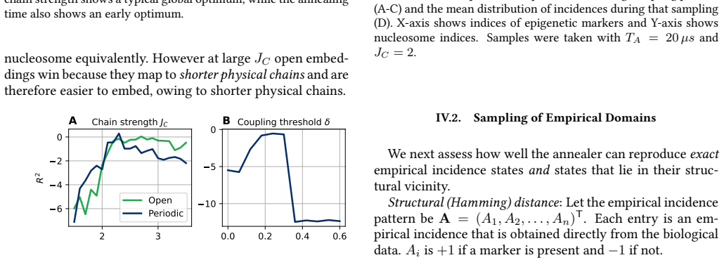
- Pruning weak couplings below a threshold near $\delta = 0.25$ simplifies the embedding and can improve performance, while pruning beyond that removes biologically relevant interactions and degrades the match.
Reading between the lines
- A testable extension the paper leaves implicit is to include the strongest mixed couplings (different markers at different nucleosomes) and re-learn the model; if $R^2$ improves on cross-marker spatial correlations, the Cartesian restriction is a genuine loss, and if not, the restriction is validated.
- If the reverse-annealing depth parameter controls how far sampled states sit from an empirical TAD, then varying it may produce an ensemble that can be compared directly with Hi-C maps of intermediate folding states, which the paper motivates but does not test.
- The reported speed-up is specific to fitting many copies of a small model on one chip; as hardware connectivity grows, the same cluster-replication idea would extend to larger $[M, N, L]$ windows, making genome-wide sampling a question of qubit count rather than algorithm redesign.
- The learned parameters come from a classical Boltzmann loop; a fully quantum loop, in which quantum annealing samples supply the gradients for parameter updates, is the natural next step and would remove the classical sampling bottleneck entirely.
Editorial analysis
A structured set of objections, weighed in public.
Referee Report
Summary. The manuscript presents a pipeline that binarizes IMR90 ChIP-seq data into 12 epigenetic markers over 200-bp bins, learns an Ising/QUBO model whose parameters are per-marker biases, intra-nucleosome marker couplings, and same-marker inter-nucleosome distance couplings, and embeds this Cartesian model onto the D-Wave Pegasus topology. The parameters are fitted by classical Boltzmann sampling against empirical mean incidences and correlations. The authors then benchmark quantum annealing samples against classical Boltzmann samples and empirical statistics, reporting qualitative agreement in Fig. 11, grid-search results for annealing time, chain strength, boundary conditions, and coupling threshold, plus reverse-annealing and cluster-parallelization experiments. The abstract claims that QA reproduces mean marker incidences and intra- and inter-nucleosome correlations while generating TAD-like structural motifs, rather than reconstructing exact TAD size distributions or insulation scores.
Significance. If the missing quantitative support were supplied, this would be a useful proof-of-concept that a D-Wave quantum annealer can sample an epigenetically learned Ising model as well as a classical Boltzmann sampler for model sizes up to [12, 25, 5]. The paper has clear strengths: an explicit QUBO mapping, a detailed embedding analysis with chain-length statistics across Pegasus and Zephyr topologies, use of real quantum hardware, and transparent hyperparameter sweeps over T_A, J_C, boundary conditions, and coupling threshold. However, the currently reported evidence is essentially qualitative: Fig. 11 has no error bars or reported R2 values, no statistical tests are given, and the omitted mixed-coupling sector is not validated. The paper also conflates model learning with hardware sampling and overstates timing gains by comparing anneal time to full Markov-chain time. These issues are fixable within the scope of the manuscript, but they must be addressed before the central claim can be accepted.
major comments (5)
- [Section II.2, Eq. (2)] The assertion that mixed marker-nucleosome couplings Q^{nn'}_{mm'} for m != m' and n != n' 'do not bear significant statistical relevance' is not supported by any reported analysis. The learning objective in Section II.4 fits only mean incidences, intra-nucleosome marker correlations, and same-marker inter-nucleosome correlations, and Fig. 11 evaluates exactly those quantities; therefore neither the learning procedure nor the evaluation can detect whether the omitted couplings are negligible. Please add the empirical cross-marker spatial correlation matrix, or a summary of its magnitude relative to the included terms, and if those correlations are non-negligible, either include the terms or demonstrate that their omission does not change the conclusions. This point is load-bearing because the Cartesian structure is what keeps the objective graph sparse enough for the minor-embedding analysis in Section III.2.
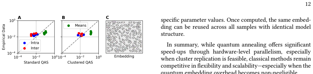
- [Figure 11 and Section IV.1] The central claim of statistical reproduction rests on a qualitative visual comparison. No error bars, confidence intervals, per-category R2 values, or statistical tests are reported; the R2 metric introduced in the grid-search paragraph is not used in Fig. 11 or in any table, and no statement about run-to-run variability is made. Please report R2 or a comparable error metric with uncertainties from repeated QA and classical runs, for each model size and statistic category, and state explicitly whether the QA-CBS differences are within noise. Because the displayed agreement is obtained after a grid search over T_A, J_C, boundary conditions, and delta, a sensitivity analysis or holdout evaluation is needed to establish that the agreement is not an artifact of parameter selection.
- [Section II.4 and Section IV.1] Because the model parameters are learned from the same empirical means and correlations that are used as the evaluation target in Fig. 11, the reproduction of these statistics by the classical Boltzmann sampler is partly by construction. For the QA claim, what is actually demonstrated is that QA sampling from the learned Hamiltonian approximates the classical sampler's target distribution. The manuscript should separate these two statements, for example by reporting QA-vs-exact-model statistics (sampled model means and correlations versus their Boltzmann expectations) in addition to QA-vs-empirical statistics. Without that separation, the abstract's phrasing that QA 'reproduces' empirical statistics conflates model learning with hardware sampling.
- [Section IV.1, Fig. 14] The claim that the sampled configurations exhibit 'TAD-like structural motifs' is supported only by three selected sample images. No automated or statistical definition of a TAD-like motif is given, no quantitative measure of motif frequency is reported, and there is no comparison with the frequency of such motifs in random configurations or in classical Boltzmann samples. Please provide a quantitative criterion for TAD-likeness, its distribution over many samples, and a null-model comparison; otherwise the motif claim remains anecdotal.
- [Section IV.3] The timing comparison is not apples-to-apples. The reported '100x' speed-up from cluster-parallelized QA counts only annealing time, while the classical side appears to include full Markov-chain step time; QPU programming, readout, and classical post-processing are not included in the quantum time. A meaningful comparison should report end-to-end wall-clock time for both methods, or explicitly qualify the speed-up as anneal-time-only and acknowledge that this does not support the 'order-of-magnitude reductions in sampling time' statement in the conclusion.
minor comments (6)
- [Introduction, first paragraph after Section I] The sentence 'QA faithfully reproduces the TAD length distributions and insulation score profiles while delivering an order-of-magnitude speedup' contradicts the abstract and Section II.3, which state that exact TAD size distributions and insulation scores are not reconstructed; please align these statements.
- [Figure 11] The figure lacks labeled axes, a legend explaining the colored categories, and a statement of whether the y-axis is on a logarithmic scale; the acronyms CBS and QAS should be expanded in the caption.
- [Figure 12] The caption text describing which panel shows chain strength and which shows annealing time appears to be swapped relative to the panel layout; please correct the description and label both axes explicitly.
- [Equations (2)-(3) and Appendix E] There are notational inconsistencies in the QUBO indices, including the conditions m > m' and n > n' in Eq. (1) versus the sums in Eq. (3), and the threshold condition in Appendix E is written as delta > max(|J_i|), which does not match the subsequent description of removing couplings below delta; please standardize the notation.
- [Section II.4 and Appendix B] Reproducibility details are missing: the binarization threshold for ChIP-seq peak strength is not specified, the Boltzmann sampling parameters (nsteps, beta, learning rate) are not given, and no data or code availability statement is provided.
- [Figures 20 and 22] There are small typos such as 'Zephr' instead of 'Zephyr' in Fig. 20, and the caption 'max(CL)' in Fig. 24 should be 'max(C_L)' or similar; please proofread the figure text.
Circularity Check
The headline statistics that QA 'reproduces' are the same statistics used as the learning target, so the empirical-statistics result is partly by construction; the TAD-template experiments likewise feed the target motif in as bias.
-
fitted input called prediction
[Section II.1 step 2, Section II.4, Section IV.1 / Fig. 11]
"Key statistics, such as the mean incidence of markers µm = 1/N Σ xn_m and correlations between markers within ρ_mm′ = 1/N Σ xn_m · xn_m′ and across nucleosomes ρ^l_m = 1/N Σ xn_m · xn+l_m, are computed to describe the dataset’s distribution and are later used to evaluate sampled chromatin states. ... Adjust the model parameters based on the discrepancy between simulated and empirical statistics."
The empirical mean incidences, intra-nucleosome correlations, and inter-nucleosome correlations are first computed in II.1 and then used as the training target of the learning procedure in II.4. The same statistics are later reported in Fig. 11 as the success metric: 'samples generated with quantum annealing reproduce chromatin statistics to the same level of accuracy as those obtained with classical Boltzmann sampling.' For the classical Boltzmann sampler, reproducing these statistics is the optimization objective, so the agreement is not an independent prediction but a fit-quality measure. The quantum annealer inherits the fitted parameters, so its agreement with empirical statistics is bounded by the quality of that fit plus hardware sampling fidelity.
-
self definitional
[Section IV.2, Figs. 15-17]
"using the incidence bias model [46], the effect of the bias strength f is examined with incidence biases taken from a data section of a promoter TAD (see figure 15). ... In all cases, key structural features of the empirical state (panel A) remain visible, demonstrating that the bias effectively confines sampling to a meaningful vicinity around the biological reference."
Here the 'TAD-like' output is produced by explicitly feeding the empirical promoter TAD into the sampler as the incidence bias, and the reported success is that the empirical state's structural features remain visible in the samples. That is close to a self-definitional check: the input template defines the motif that is recovered. The reverse-annealing variant makes this even more direct, since 'the system begins in a classical state aligned with the empirical template.' Showing that biased sampling stays near the bias is a demonstration of the biasing mechanism, but it is not independent evidence that the unbiased model generates TAD-like motifs.
full rationale
The paper's genuinely new and non-circular content is the hardware engineering: embedding the learned Cartesian QUBO on Pegasus, measuring chain lengths, tuning annealing time and chain strength, and showing that D-Wave samples approximate the fitted Boltzmann distribution about as well as classical Boltzmann sampling. None of that requires assuming the biology it claims to reproduce. The circularity is partial and confined to the validation framing. The statistics used for evaluation in Fig. 11 are exactly the statistics minimized in the learning loop of II.4, so for the classical sampler the agreement is by construction (up to optimization convergence), and for the quantum sampler it is a hardware-fidelity test of a fitted model rather than a predictive test of the epigenetic model. Similarly, the TAD-motif demonstrations in IV.2 inject the empirical TAD as a bias or initial state, so recovering its features is expected. The Cartesian exclusion of mixed marker-nucleosome couplings (Eq. 2) is an unsupported modeling assumption and a correctness risk, but it is not circularity. The paper's self-citations (e.g., refs. [26,27,29,36,37,40,41,46]) are methodological or technical and are not load-bearing evidence for the central sampling claim; the model framework is attributed to ref. [23], not to the authors' own prior work. Overall, the central 'reproduces statistics' claim reduces partly to its own training objective, but the paper does not hide this and it does provide an independent hardware benchmarking result, so the appropriate score is moderate rather than extreme.
Assumptions & free parameters
free parameters (7)
- QUBO bias q_m
- Intra-nucleosome couplings R_{mm'}
- Inter-nucleosome couplings S^l_m
- Annealing time T_A =
20 us used in examples; grid searched
- Chain strength J_C =
2 used in examples; grid searched
- Coupling threshold delta =
about 0.25 safe window
- Bias strength f =
5 used in examples
assumptions (8)
- standard math Ising and QUBO models are equivalent and both can be sampled from a Boltzmann distribution.
- standard math The adiabatic theorem guarantees that slow annealing keeps the system near the instantaneous ground state.
- domain assumption Each 200 bp bin corresponds to one nucleosome and binarization captures the relevant epigenetic state.
- domain assumption Only intra-nucleosome marker couplings and same-marker inter-nucleosome couplings are relevant; mixed couplings are zero (Eq. 2).
- domain assumption Model parameters are translationally invariant across nucleosome positions.
- domain assumption The learned pairwise statistics are sufficient to generate TAD-like structures.
- ad hoc to paper Coupling strength threshold delta preserves biologically relevant interactions within a safe window.
- ad hoc to paper Bias f and reverse annealing parameters can steer sampling near a template state without corrupting the model.
Cite this review
Pith. "Pith review of Intermediate State Formation of Topologically Associated Chromatin Domains using Quantum Annealing." pith.science (2026). https://pith.science/paper/7XSKCHRN
@misc{pith2026250523289,
  author       = {Pith},
  title        = {Pith review of: Intermediate State Formation of Topologically Associated Chromatin Domains using Quantum Annealing},
  year         = {2026},
  howpublished = {\url{https://pith.science/paper/7XSKCHRN}},
  note         = {Machine review of arXiv:2505.23289}
}
read the original abstract
Topologically Associating Chromatin Domains are spatially distinct chromatin regions that regulate transcription by segregating active and inactive genomic elements. Empirical studies show that their formation correlates with local patterns of epigenetic markers, yet the precise mechanisms linking 1D epigenetic landscapes to 3D chromatin folding remain unclear. Recent models represent chromatin as a spin system, where nucleosomes are treated as discrete-state variables coupled by interaction strengths derived from genomic and epigenetic data. Classical samplers struggle with these models due to high frustration and dense couplings. Here, we present a quantum annealing (QA) approach to efficiently sample chromatin states, embedding an epigenetic Ising model into the topology of D-Wave quantum processors. Rather than reconstructing exact TAD size distributions or insulation scores, our method reproduces statistical features, such as mean marker incidences and intra-/inter-nucleosome correlations, while generating configurations that exhibit TAD-like structural motifs. These results demonstrate QA as an alternative to explore the chromatin architecture and provide a foundation in epigenetic modeling.
Figures


Figures from the paper (19 more)






Reference graph
Works this paper leans on
-
[1]
In the chromatin struc- ture, each nucleosome corresponds to a 200 base-pair section of DNA
Binarization: Since the model is based on binary inci- dences of epigenetic markers on different nucleosome locations, we first binarize and—for better computa- tional efficiency—bin the (semi-)continuous format of epigenetic markers in [30, 31]. In the chromatin struc- ture, each nucleosome corresponds to a 200 base-pair section of DNA. For example, the ...
-
[2]
Statistics: We compute statistical features of bina- rized empiric data as a reference for the learning pro- cedure and later sampling results. The binarized data is represented as a binary matrix A, where each el- ement indicates the presence (1) or absence (0) of a marker at a specific nucleosome position. The indi- vidual incidence cells are addressed ...
-
[3]
We parameterize the model to accurately produce the given statistics during sam- pling
Model: We define a model based on epigenetic marker incidences that maps probable chromatin states ac- cording to the recorded statistics to low-energy values of an objective function. We parameterize the model to accurately produce the given statistics during sam- pling. Until now, these steps have been required for both clas- sical and quantum sampling....
-
[4]
H3K27ac, CpG-methylation) is present ( 1) or ab- sent (0) at nucleosome position n
Objective: In our binary incidence tensorx, each vari- able x n m ∈ {0, 1} records whether epigenetic markerm (e.g. H3K27ac, CpG-methylation) is present ( 1) or ab- sent (0) at nucleosome position n. We define an objec- tive function in a consistent way with the model en- coded in the energy expectation of the quantum sys- tem’s Hamiltonian: H(x) = X m≥m′...
-
[5]
Embedding: We need to embed the objective Hamil- tonian onto the quantum processor’s specific topology in a D-Waves quantum annealing device
-
[6]
Sampling: Using the parameters computed in step 3, we sample the states and anneal multiple times with the quantum annealer
-
[7]
Analysis: We compare and analyze the statistics of samples from quantum annealers with the data set of chromatin-state empiric statistics. II.2. QUBO Objectives As discussed above, our binary incidence tensor x n m ∈ {0, 1} records whether epigenetic marker m is present ( 1) or absent (0) at nucleosome position n. When this tensor is assigned to an uncons...
-
[8]
Highly specific models: One can design a model that cap- tures local biases and correlations directly from the empirical data, effectively mapping each variable in the model to a spe- cific genomic location. In this case, quantum sampling yields very few states that differ from the empirical configuration, making it unsuitable for generating diverse alter...
Show all 76 references
-
[9]
Starting from a random point in parameter space ensures explo- ration of diverse regions in the optimization landscape
Initialize the model with random parameters. Starting from a random point in parameter space ensures explo- ration of diverse regions in the optimization landscape
-
[10]
Sampling generates configurations according to the current model’s energy landscape, mimicking physical equilibrium behavior
Generate multiple samples from the model using Boltz- mann sampling. Sampling generates configurations according to the current model’s energy landscape, mimicking physical equilibrium behavior
-
[11]
Quantities such as marginal probabilities and pairwise correlations are calculated to compare with empirical data
Compute statistical observables from the generated samples. Quantities such as marginal probabilities and pairwise correlations are calculated to compare with empirical data
-
[12]
The differ- ence between the observed and simulated statistics de- fines a loss function, minimized by updating the pa- rameters
Adjust the model parameters based on the discrepancy between simulated and empirical statistics. The differ- ence between the observed and simulated statistics de- fines a loss function, minimized by updating the pa- rameters
-
[13]
The iteration continues until the model statistically reproduces key features of the empirical dataset
Repeat steps 2–4 until the total error falls below a threshold. The iteration continues until the model statistically reproduces key features of the empirical dataset. The Boltzmann Sampling works with the following steps:
-
[14]
Start with a random model state
-
[15]
One vari- able is selected for a potential update, in line with a typical Metropolis scheme
Randomly select the incidence of the model. One vari- able is selected for a potential update, in line with a typical Metropolis scheme
-
[16]
This step quanti- fies how the configuration’s energy would change if the variable were flipped
Compute the energy difference ∆E resulting from flip- ping the selected incidence variable. This step quanti- fies how the configuration’s energy would change if the variable were flipped
-
[17]
Energy-lowering moves are always accepted; energy-increasing ones are accepted with a probability based on ∆E
Update the variable with probability P = e−β∆E if ∆E ≥ 0, and withP = 1 if ∆E <0. Energy-lowering moves are always accepted; energy-increasing ones are accepted with a probability based on ∆E
-
[18]
The process con- tinues for a predefined number of steps to ensure ade- quate mixing of the state space
Repeat steps 2–4 for nsteps iterations. The process con- tinues for a predefined number of steps to ensure ade- quate mixing of the state space. 5 6 qi 0.0 0.5 1.0 1.5 2.0 2.5 3.0Counts 2 0 Rmm′ 0 2 4 6 8 0.50 0.25 Sl m 0.0 2.5 5.0 7.5 10.0 12.5 FIG. 4. Frequency of QUBO param...
-
[19]
Marker intersection graph IM : This graph is con- structed by grouping all edges associated with the same nucleosom but between all different markers. Since each marker is allowed to interact with every other marker within the same nucleosome, the result- ing graph is a comple...
-
[20]
is markerm present on nucleosome n?
Nucleosome intersection graph IN : This graph is built from sets of edges associated with each nucleo- some’s connections to others. For a model with local inter-nucleosomic interactions (up to a fixed distance L), the graph becomes a cyclic 2L-regular graph (see Fig. 8B). In ...
-
[21]
Dna methylation: an epigenetic mark of cellular memory,
M. Kim and J. Costello, “Dna methylation: an epigenetic mark of cellular memory, ”Experimental & Molecular Medicine , vol. 49, pp. e322–e322, Apr 2017
2017
-
[22]
Transgenerational epigenetic in- heritance: Myths and mechanisms,
E. Heard and R. Martienssen, “Transgenerational epigenetic in- heritance: Myths and mechanisms, ”Cell, vol. 157, no. 1, pp. 95– 109, 2014
2014
-
[23]
Mater- nal–infant interaction quality is associated with child nr3c1 cpg site methylation at 7 years of age,
E. A. Holdsworth, L. M. Schell, and A. A. Appleton, “Mater- nal–infant interaction quality is associated with child nr3c1 cpg site methylation at 7 years of age, ” American Journal of Human Biology, vol. n/a, no. n/a, p. e23876, 2023
2023
-
[24]
R. Paro, U. Grossniklaus, R. Santoro, and A. Wutz, Introduction to Epigenetics. Switzerland: Springer Cham, 2021
2021
-
[25]
Chromatin Domains: the Unit of Chromosome Organization,
D. U. G. Jesse R. Dixon and B. Ren, “Chromatin Domains: the Unit of Chromosome Organization, ” Molecular Cell , vol. 62, p. 668–680, 06 2016
2016
-
[26]
Formation of new chromatin domains deter- mines pathogenicity of genomic duplications,
M. F. et al., “Formation of new chromatin domains deter- mines pathogenicity of genomic duplications, ”Nature, vol. 538, p. 265–269, 10 2016
2016
-
[27]
Demonstration of a scaling advan- tage for a quantum annealer over simulated annealing,
T. Albash and D. A. Lidar, “Demonstration of a scaling advan- tage for a quantum annealer over simulated annealing, ”Physi- cal Review X, vol. 8, no. 3, p. 031016, 2018
2018
-
[28]
Comparative study of the performance of quantum annealing and simulated anneal- ing,
H. Nishimori, J. Tsuda, and S. Knysh, “Comparative study of the performance of quantum annealing and simulated anneal- ing, ”Physical Review E, vol. 91, no. 1, p. 012104, 2015
2015
-
[29]
Folding lattice proteins with quantum annealing,
A. Irbäck, L. Knuthson, S. Mohanty, and C. Peterson, “Folding lattice proteins with quantum annealing, ”Phys. Rev. Res., vol. 4, p. 043013, Oct 2022
2022
-
[30]
Using quantum annealing to design lattice proteins,
A. Irbäck, L. Knuthson, S. Mohanty, and C. Peterson, “Using quantum annealing to design lattice proteins, ” Phys. Rev. Res., vol. 6, p. 013162, Feb 2024
2024
-
[31]
Efficient quantum algorithm for lat- tice protein folding,
Y. Wang and X. Zhou, “Efficient quantum algorithm for lat- tice protein folding, ”Quantum Science and Technology, vol. 10, no. 1, p. 015056, 2024
2024
-
[32]
Rna folding using quantum computers,
D. M. Fox, C. M. MacDermaid, A. M. Schreij, M. Zwierzyna, and R. C. Walker, “Rna folding using quantum computers, ” PLOS Computational Biology, vol. 18, no. 4, p. e1010032, 2022
2022
-
[33]
A qubo model of the rna folding problem optimized by varia- tional hybrid quantum annealing,
T. Zaborniak, J. Giraldo, H. Müller, H. Jabbari, and U. Stege, “A qubo model of the rna folding problem optimized by varia- tional hybrid quantum annealing, ” in 2022 IEEE International Conference on Quantum Computing and Engineering (QCE) , pp. 174–185, IEEE, 2022
2022
-
[34]
Predicting rna secondary structure on univer- sal quantum computer,
J. Jiang, Q. Yan, Y. Li, M. Lu, Z. Cui, M. Dou, Q. Wang, Y.-C. Wu, and G.-P. Guo, “Predicting rna secondary structure on univer- sal quantum computer, ”arXiv preprint arXiv:2305.09561, 2023
2023 arXiv
-
[35]
Designing peptides on a quantum computer,
V. K. Mulligan, H. Melo, H. I. Merritt, S. Slocum, B. D. Weitzner, A. M. Watkins, P. D. Renfrew, C. Pelissier, P. S. Arora, and R. Bonneau, “Designing peptides on a quantum computer, ” BioRxiv, p. 752485, 2019
2019
-
[36]
Quantum annealing designs nonhemolytic antimi- crobial peptides in a discrete latent space,
A. Tucs, F. Berenger, A. Yumoto, R. Tamura, T. Uzawa, and K. Tsuda, “Quantum annealing designs nonhemolytic antimi- crobial peptides in a discrete latent space, ” ACS Medicinal Chemistry Letters, vol. 14, no. 5, pp. 577–582, 2023
2023
-
[37]
Sampling a rare pro- tein transition using quantum annealing,
D. Ghamari, R. Covino, and P. Faccioli, “Sampling a rare pro- tein transition using quantum annealing, ”Journal of Chemical Theory and Computation, vol. 20, no. 8, pp. 3322–3334, 2024
2024
-
[38]
Complexity of chromatin fold- ing is captured by the strings and binders switch model,
M. Barbieri, M. Chotalia, J. Fraser, L.-M. Lavitas, J. Dostie, A. Pombo, and M. Nicodemi, “Complexity of chromatin fold- ing is captured by the strings and binders switch model, ”Proc. Natl. Acad. Sci. U. S. A. , vol. 109, pp. 16173–16178, Oct. 2012
2012
-
[39]
The 3D genome as moderator of chro- mosomal communication,
J. Dekker and L. Mirny, “The 3D genome as moderator of chro- mosomal communication, ”Cell, vol. 164, pp. 1110–1121, Mar. 2016
2016
-
[40]
Chromatin insulators: Linking genome organization to cellular function,
J. E. Phillips-Cremins and V. G. Corces, “Chromatin insulators: Linking genome organization to cellular function, ” Mol. Cell , vol. 50, pp. 461–474, May 2013
2013
-
[41]
Structural modeling of chromatin integrates genome features and reveals chromosome folding principle,
W. J. Xie, L. Meng, S. Liu, L. Zhang, X. Cai, and Y. Q. Gao, “Structural modeling of chromatin integrates genome features and reveals chromosome folding principle, ” Scientific Reports , vol. 7, p. 2818, June 2017
2017
-
[42]
Identifi- cation of alternative topological domains in chromatin,
D. Filippova, R. Patro, G. Duggal, and C. Kingsford, “Identifi- cation of alternative topological domains in chromatin, ”Algo- rithms Mol. Biol., vol. 9, Jan. 2014
2014
-
[43]
Learning mechanism of chromatin domain formation with big data,
W. J. Xie and B. Zhang, “Learning mechanism of chromatin domain formation with big data, ”bioRxiv, 2018
2018
-
[44]
Probabilistic modelling of chromatin code landscape reveals functional diversity of enhancer-like chromatin states,
J. Zhou and O. G. Troyanskaya, “Probabilistic modelling of chromatin code landscape reveals functional diversity of enhancer-like chromatin states, ”Nature communications, vol. 7, no. 1, p. 10528, 2016
2016
-
[45]
Global quantitative modeling of chromatin factor interactions,
J. Zhou and O. G. Troyanskaya, “Global quantitative modeling of chromatin factor interactions, ”PLoS computational biology , vol. 10, no. 3, p. e1003525, 2014
2014
-
[46]
Entropy pro- duction in quantum is different,
M. H. Ansari, A. van Steensel, and Y. V. Nazarov, “Entropy pro- duction in quantum is different, ”Entropy, vol. 21, no. 9, p. 854, 2019
2019
-
[47]
Exact correspondence be- tween renyi entropy flows and physical flows,
M. H. Ansari and Y. V. Nazarov, “Exact correspondence be- tween renyi entropy flows and physical flows, ”Physical Review B, vol. 91, no. 17, p. 174307, 2015
2015
-
[48]
Error mitigation of entangled states using brainbox quantum autoencoders,
J. Pazem and M. H. Ansari, “Error mitigation of entangled states using brainbox quantum autoencoders, ” arXiv preprint arXiv:2303.01134, 2023
2023
-
[49]
Error mitigation in brainbox quan- tum autoencoders,
J. Pazem and M. H. Ansari, “Error mitigation in brainbox quan- tum autoencoders, ” Scientific Reports , vol. 15, no. 1, p. 2257, 2025
2025
-
[50]
Roadmap epigenomics project
NIH Roadmap Epigenomics Mapping Consortium, “Roadmap epigenomics project. ” https://egg2.wustl.edu/ roadmap/web_portal/. Accessed: 2023-01-10
2023
-
[51]
Characterization of a new human diploid cell strain, IMR-90,
W. W. Nichols, D. G. Murphy, V. J. Cristofalo, L. H. Toji, A. E. Greene, and S. A. Dwight, “Characterization of a new human diploid cell strain, IMR-90, ” Science, vol. 196, pp. 60–63, Apr. 1977
1977
-
[52]
(meaning that states that only differ by a periodic shift in nu- cleosome positions produce the same objective energy)
-
[53]
Coherent quan- tum annealing in a programmable 2,000 qubit ising chain,
A. D. King, S. Suzuki, J. Raymond, A. Zucca, T. Lanting, F. Al- tomare, A. J. Berkley, S. Ejtemaee, E. Hoskinson, S. Huang, E. Ladizinsky, A. J. R. MacDonald, G. Marsden, T. Oh, G. Poulin- Lamarre, M. Reis, C. Rich, Y. Sato, J. D. Whittaker, J. Yao, R. Har- ris, D. A. Lidar, H...
2022
-
[54]
Computational supremacy in quantum simulation,
A. D. King, A. Nocera, M. M. Rams, J. Dziarmaga, R. Wiersema, W. Bernoudy, J. Raymond, N. Kaushal, N. Heinsdorf, R. Har- ris, et al., “Computational supremacy in quantum simulation, ” arXiv preprint arXiv:2403.00910, 2024. 14
2024
-
[55]
Quantum an- nealing for industry applications: Introduction and review,
S. Yarkoni, E. Raponi, T. Bäck, and S. Schmitt, “Quantum an- nealing for industry applications: Introduction and review, ”Re- ports on Progress in Physics , vol. 85, no. 10, p. 104001, 2022
2022
-
[56]
The effect of environmental coupling on tunneling of quasiparticles in josephson junctions,
M. H. Ansari, F. K. Wilhelm, U. Sinha, and A. Sinha, “The effect of environmental coupling on tunneling of quasiparticles in josephson junctions, ” Superconductor Science and Technology , vol. 26, no. 12, p. 125013, 2013
2013
-
[57]
Suppression of unwanted zz inter- actions in a hybrid two-qubit system,
J. Ku, X. Xu, M. Brink, D. C. McKay, J. B. Hertzberg, M. H. Ansari, and B. Plourde, “Suppression of unwanted zz inter- actions in a hybrid two-qubit system, ” Physical review letters , vol. 125, no. 20, p. 200504, 2020
2020
-
[58]
Prospects for quantum enhancement with diabatic quantum annealing,
E. Crosson and D. Lidar, “Prospects for quantum enhancement with diabatic quantum annealing, ” Nature Reviews Physics , vol. 3, no. 7, pp. 466–489, 2021
2021
-
[59]
Why adiabatic quantum annealing is unlikely to yield speed-up,
A. Villanueva, P. Najafi, and H. J. Kappen, “Why adiabatic quantum annealing is unlikely to yield speed-up, ” 2022
2022
-
[60]
Zz freedom in two-qubit gates,
X. Xu and M. Ansari, “Zz freedom in two-qubit gates, ”Physical review applied, vol. 15, no. 6, p. 064074, 2021
2021
-
[61]
Lattice hamiltonians and stray interactions within quantum processors,
X. Xu, Manabputra, C. Vignes, M. H. Ansari, and J. M. Martinis, “Lattice hamiltonians and stray interactions within quantum processors, ”Physical Review Applied , vol. 22, no. 6, p. 064030, 2024
2024
-
[62]
Cluster graph modifica- tion problems,
R. Shamir, R. Sharan, and D. Tsur, “Cluster graph modifica- tion problems, ”Discrete Applied Mathematics , vol. 144, no. 1, pp. 173–182, 2004. Discrete Mathematics and Data Mining
2004
-
[63]
In our setting, sets are defined by the connectivity of markers or nu- cleosomes
In general, an intersection graph is a graph where each node represents a set, and an edge exists between two nodes if the corresponding sets have a non-empty intersection [48]. In our setting, sets are defined by the connectivity of markers or nu- cleosomes
-
[64]
Note that the typical graph theory definition of a graph diam- eter refers to the longest path, not the number of nodes in the longest path (i.e. +1)
-
[65]
Programming the D-Wave QPU: Setting the Chain Strength,
D.-W. Systems, “Programming the D-Wave QPU: Setting the Chain Strength, ” Tech. Rep. 14-1041A-A, D-Wave Systems Inc., 3033 Beta Ave, Burnaby, BC V5G 4M9, Canada, Apr. 2020
2020
-
[66]
Intermediate state prediction in the formation of topologically associated chromatin domains using quantum annealing,
T. Kempe, “Intermediate state prediction in the formation of topologically associated chromatin domains using quantum annealing, ” 2024
2024
-
[67]
Reverse Quantum Annealing for Local Refine- ment of Solutions,
D.-W. Systems, “Reverse Quantum Annealing for Local Refine- ment of Solutions, ” Tech. Rep. 14-1018A-A, D-Wave Systems Inc., 3033 Beta Ave, Burnaby, BC V5G 4M9, Canada, Nov. 2017
2017
-
[68]
The representation of a graph by set intersections,
P. Erdös, A. W. Goodman, and L. Pósa, “The representation of a graph by set intersections, ”Canadian Journal of Mathematics , vol. 18, p. 106–112, 1966
1966
-
[69]
Fast clique minor genera- tion in chimera qubit connectivity graphs,
K. Boothby, A. D. King, and A. Roy, “Fast clique minor genera- tion in chimera qubit connectivity graphs, ” 2015
2015
-
[70]
Adiabatic quan- tum programming: Minor embedding with hard faults,
C. Klymko, B. D. Sullivan, and T. S. Humble, “Adiabatic quan- tum programming: Minor embedding with hard faults, ” 2012
2012
-
[71]
Quan- tum annealing: An overview,
A. Rajak, S. Suzuki, A. Dutta, and B. K. Chakrabarti, “Quan- tum annealing: An overview, ”Philosophical Transactions of the Royal Society A, vol. 381, no. 2241, p. 20210417, 2023
2023
-
[72]
Next-Generation Topology of D-Wave Quantum Proces- sors,
Kelly Boothby and Paul Bunyk and Jack Raymond and Aidan Roy, “Next-Generation Topology of D-Wave Quantum Proces- sors, ” tech. rep., D-Wave Systems Inc., 3033 Beta Ave, Burnaby, BC V5G 4M9, Canada, Feb. 2020
2020
-
[73]
Bi- nary utilities directory
University of California Santa Cruz Genomics Institute, “Bi- nary utilities directory. ” http://hgdownload.soe. ucsc.edu/admin/exe/linux.x86_64/. Accessed: 2023-03-04
2023
-
[74]
A practical heuristic for finding graph minors,
J. Cai, W. G. Macready, and A. Roy, “A practical heuristic for finding graph minors, ” 2014
2014
-
[75]
The argument also holds for Ising parameters, since the cou- plings are only scaled with a constant factor during the con- version
-
[76]
Qpu-specific characteristics
D-Wave Systems Inc., “Qpu-specific characteristics. ” https://docs.dwavesys.com/docs/latest/ doc_physical_properties.html, 2023. Accessed: 2023-04-26. 15 Appendix A: Embedding on D-Wave Topology Based on the objective Hamiltonian, the required logical couplings between qubits ...
2023
Reviewed August 7, 2026 · model on record in the stance chip above.
Discussion (0). Continue with ORCID to comment.