REVIEW 2 major objections 5 minor 65 references
For measurement-based GHZ preparation, optimal decoding means maximizing the expected squared magnetization of the corrected state—and a syndrome-weighted matching algorithm comes within 87% of that ideal.
Reviewed by Pith at T0; open to challenge. T0 means a machine referee read the full paper against a public rubric. the ladder, T0–T4 →
T0 review · deepseek-v4-flash
2026-08-04 01:11 UTC pith:A4OQDL5V
load-bearing objection The practical result—syndrome-weighted MWPM—is real and useful, but the 'optimal decoder' branding outruns the certification, and the off-diagonal gap-closing percentages sit on a yardstick the authors themselves flag as unresolved. the 2 major comments →
Optimal Decoding for Measurement-Based GHZ State Preparation: The Maximum-Utility Decoder
The pith
A machine-rendered reading of the paper's core claim, the machinery that carries it, and where it could break.
Core claim
The central claim is that a decoder for measurement-based GHZ state preparation should maximize the expected squared magnetization ⟨M̂²⟩ of the corrected state rather than the probability of a correct logical recovery. Because the bit-flip correction τ enters only through τ_i σ_i, the expected utility is exactly the quadratic form (1/N²) τᵀ C(s) τ, where C_ij(s) = ⟨σ_i σ_j⟩_s is the spin-spin correlation matrix of the random-bond Ising model conditioned on the measured syndromes. Maximizing this form is the maximum-utility decoder (MUD); the paper shows it attains the highest possible per-shot decoded order. For scalability, the paper proposes a syndrome-weighted MWPM whose edge weights depe
What carries the argument
The central object is the maximum-utility decoder (MUD): given a measured syndrome configuration s, it returns the correction τ maximizing the expected squared magnetization, which reduces to maximizing τᵀ C(s) τ with C_ij(s)=⟨σ_i σ_j⟩_s, a quadratic unconstrained binary optimization (QUBO) problem. Two concrete mechanisms carry the scalable approximation. First, syndrome-weighted MWPM assigns each edge a weight w_ij = J_+ (if s_ij=1) or |J_-| (if s_ij=-1), so the matching distinguishes ferromagnetic from antiferromagnetic bonds and removes most of the degeneracy of shortest correction paths. Second, a convolutional neural network takes the syndrome and the baseline correction chain as input
Load-bearing premise
The benchmark 'optimal threshold' used to measure near-optimality is the decoder-independent entanglement transition; if that entanglement threshold is not, in fact, the best achievable decoding threshold—something the paper's own finite-size extrapolation of the exact MUD hints at—then the reported closing fractions overestimate how close the scalable decoders come to optimal.
What would settle it
Extrapolate the exact MUD threshold to the thermodynamic limit using improved finite-size scaling (larger L via truncated MUD or better fits) along a fixed cut such as t_B=0.7 π/4; if the extrapolated MUD threshold lies clearly above the entanglement threshold extracted from I_c and C^(2)_c, then the entanglement benchmark is not the true decoding optimum and the reported 86% gap-closing overstates near-optimality. Alternatively, measure the MWPM threshold at two points with identical sin(2t_A) sin(2t_B); disagreement beyond numerical error would refute the leading-order gauge-oblivious bounda
If this is right
- Away from the Nishimori line, the full syndrome configuration carries decoding information that gauge-invariant fluxes alone discard; weighting matching edges by syndrome sign exploits this at no extra cost beyond bare MWPM.
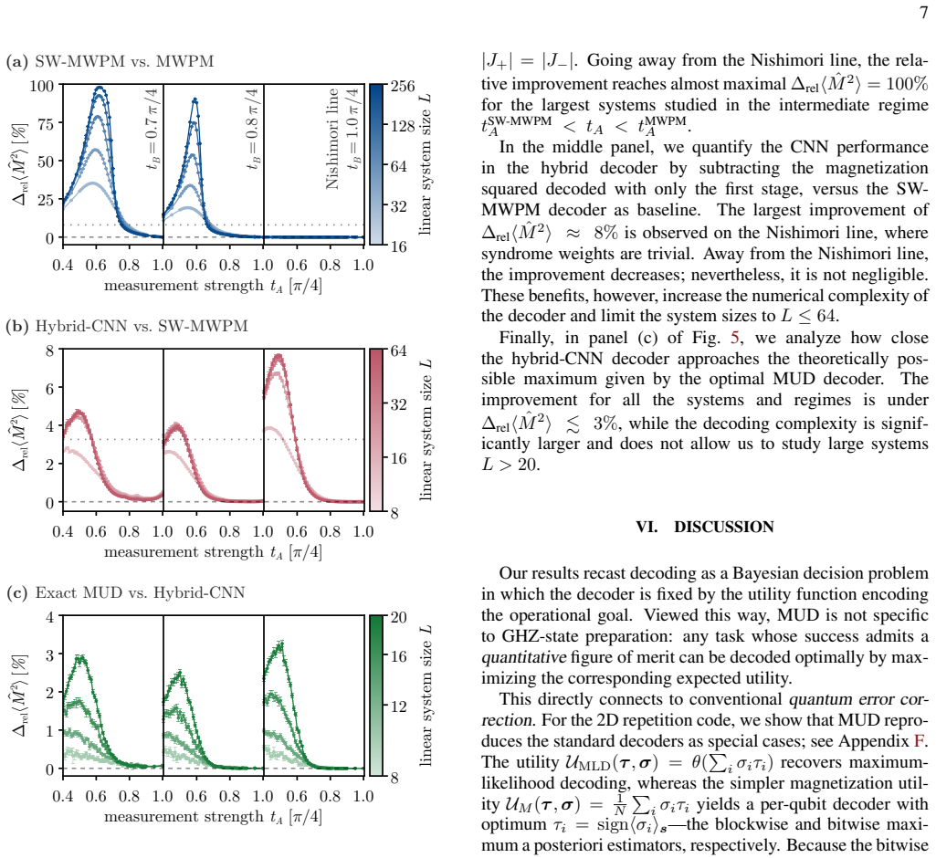
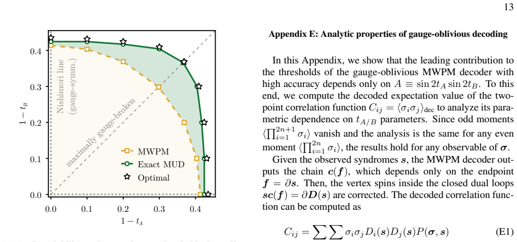
- At N=256×256, the syndrome-weighted first stage alone closes up to 87% of the threshold gap between bare MWPM and the optimal entanglement-limited value, with the largest gain on the maximally gauge-broken diagonal t_A=t_B.
- The hybrid-CNN decoder restores additional long-range order, especially on the Nishimori line where syndrome weights are trivial, and comes within about 3% of the exact MUD across the studied range.
- Because MUD reduces to MWPM or MLD for binary utilities, the maximum-utility framework generalizes standard surface-code decoding and can be re-targeted by redefining the utility function, e.g., to bitwise MAP or operation-tailored goals.
- The phase boundary of any gauge-oblivious decoder is set by the product sin(2t_A) sin(2t_B) = const to leading order, so threshold curves in the (t_A,t_B) plane should be circular around the strong-measurement point.
Where Pith is reading between the lines
- The paper's near-optimality percentages use the decoder-independent entanglement threshold as the 'optimal' benchmark; the paper itself notes in Appendix D that its extrapolated exact-MUD threshold appears somewhat larger than that entanglement value, so the 87% figure could be an overestimate—or a hint of a genuine decodability–entanglement separation.
- A direct test of the leading-order gauge-oblivious prediction: two parameter points (t_A,t_B) with the same value of sin(2t_A) sin(2t_B) should have identical MWPM thresholds up to corrections of order 10⁻³; measuring the difference would isolate gauge-symmetry breaking effects.
- The utility-maximization framing suggests a design principle beyond GHZ states: for any decoding task with a continuous figure of merit—logical-gate fidelity, operation success probability, metrological sensitivity—one can define a custom utility and use the same QUBO-plus-refinement pipeline, with hardware noise in the feedback itself folded into the utility.
- Because the bitwise magnetization utility yields the simple rule τ_i = sign⟨σ_i⟩_s and avoids the Heaviside nonlinearity of blockwise MLD, it is plausible that bitwise MUD delivers competitive logical fidelity at a fraction of the cost; the paper leaves this quantitative comparison for future work.
Editorial analysis
A structured set of objections, weighed in public.
Referee Report
Summary. The paper frames decoding for measurement-based GHZ state preparation as minimum Bayesian risk inference with a continuous utility, specifically the squared magnetization of the decoded state. It shows that maximizing this utility is equivalent to a QUBO problem over the spin-spin correlation matrix, constructs an exact 'maximum-utility decoder' (MUD) for small systems, and proposes two scalable approximations: syndrome-weighted MWPM (SW-MWPM) and a hybrid CNN-refined decoder. The central quantitative claims are that SW-MWPM closes up to 87% of the threshold gap between bare MWPM and the optimal decoder, and that the hybrid-CNN decoder is within a few percent of the exact MUD's squared magnetization.
Significance. If the results hold, the maximum-utility framework is a genuinely useful generalization of decoding: it replaces binary logical-recovery utilities with a continuous, operationally motivated figure of merit and reduces to MLD/MWPM in known limits. The clean change of variables in App. A 1, the exact QUBO reformulation, the analytic gauge-oblivious threshold curve in App. E, and the large-scale SW-MWPM simulations are notable strengths. The numerical data are promised on Zenodo, and the paper is transparent about several finite-size and certification limitations. However, the headline 'near-optimal' threshold claim depends on an unresolved choice of benchmark, and the abstract's blanket 'highest possible per-shot' claim is stronger than the implemented certification procedure supports. These issues are local and repairable, but they affect the paper's central quantitative message.
major comments (2)
- [Eq. (17), Sec. V B, Apps. C-D] The central quantitative claim that SW-MWPM closes 86/85/64% of the gap to the optimal threshold for t_B=0.7/0.8/0.9 uses t_c^opt obtained from the decoder-independent entanglement transition (App. C). Yet App. D and Fig. 12 report that the extrapolated exact-MUD threshold does not coincide with this entanglement threshold away from t_A=t_B, and the paper itself states that the discrepancy is unresolved (linear-extrapolation curvature vs. a genuine separation). Eq. (17)'s denominator is therefore not established as the threshold of the decoder that maximizes the paper's own utility function. The diagonal 87% value is protected because the two benchmarks agree there, but the phase-diagram-wide 'near-optimal' statement and the 86/85/64% numbers are not robustly anchored. Please report T relative to the exact-MUD threshold where available, or explicitly treat the entanglement value as a bou
- [Abstract, Sec. IV A, App. A 2] The abstract claims the algorithm 'achieves the highest possible per-shot decoded quantum order.' The exact MUD is the argmax of the expected utility by definition, but the implemented solver solves an NP-hard QUBO: the local-search solution is certified only when the S matrix is positive semidefinite, and the certificate fails on 19.8%, 28.7%, and 27.0% of samples for L=8, 16, and 20, with branch-and-bound allowed to terminate without a proof. Thus the implemented decoder is not always proven to attain the global maximum. Please qualify the optimality claim (e.g., 'provably optimal in all certified cases; otherwise a heuristic') or provide additional verification for the uncertified instances, especially in the parameter regime where the GHZ state is recoverable.
minor comments (5)
- [Eq. (17)] Define t_c^opt explicitly for the one-dimensional cuts: as written, it appears to be a point in the (t_A,t_B) plane rather than a threshold on a fixed-t_B sweep.
- [Figs. 2 and 4] State explicitly in all captions that measurement strengths are in units of pi/4 and that axes such as 1-t_A and 1-t_B run from strong measurement at 0 to weak measurement at the opposite corner.
- [App. D] The statement that the data for the optimal decoding threshold 'seem to have a little curvature' should be quantified. A short discussion of alternative extrapolation forms (e.g., including a quadratic term or restricting to larger L) would strengthen confidence in the threshold estimates used in Eq. (17).
- [Sec. V B] The phrase 'the threshold is an intrinsic property of a given decoder' is slightly misleading: the threshold is decoder-dependent and is extracted through finite-size extrapolation. Consider rewording to 'the threshold for a given decoder.'
- [Footnote [36]] The footnote equates a shot fidelity of 1 with <M^2>=1, but the relation to the standard state fidelity for mixed decoded states is not spelled out. A one-sentence clarification would help readers connect the utility to conventional figures of merit.
Circularity Check
No significant circularity: the optimality claim is an explicitly derived consequence of the chosen utility, and the benchmark comparisons are external to the MUD construction.
full rationale
The paper's central identity, Eq. (A6) (equivalently Eqs. (9)-(13)), shows that the decoded squared magnetization equals the expected utility E[U] for the utility U(τ,σ)=(1/N Σ σ_i τ_i)^2. The maximum-utility decoder is then defined as the maximizer of this expected utility, so the statement that it achieves the highest possible expected ⟨M̂²⟩ is a direct consequence of the definition and is presented as such, not as an empirical prediction. The comparisons are not forced: bare MWPM minimizes a different objective (syndrome-chain weight), and SW-MWPM's weights are derived from the fully-polarized-energy expression, Eq. (14), with no fitting to the optimal decoder's output. The CNN is trained to maximize the same utility using simulated labels σ from the joint distribution, which is standard supervised learning rather than a fitted parameter being renamed as a prediction. The 'optimal threshold' benchmark used in Eq. (17) is the decoder-independent entanglement transition computed in Appendix C; it is external to the utility-maximization construction. Appendix D openly reports that the exact-MUD threshold lies above this entanglement threshold away from the diagonal and states that the source of the discrepancy is unresolved; this is a benchmark-accuracy caveat, not a circular step. Self-citations (e.g., Refs. [25], [52], [54], [38]) provide background models and numerical methods, but the key derivations and calculations are reproduced in the present paper (Appendices A-E), and no uniqueness theorem or ansatz is imported from the authors' prior work to force the central result. No step in the derivation reduces by construction to its own input beyond the transparent definitional optimality of MUD.
Axiom & Free-Parameter Ledger
free parameters (4)
- Correlation-matrix truncation radius r_max (truncated MUD) =
4 (lattice spacings)
- CNN learned weights and loss-schedule hyperparameters =
990,401 parameters; λ ramp (0.3,0.3,0.2)→(1.0,0.02,0.04)
- Nishimori error rate p_c imported for the gauge-oblivious threshold curve =
0.103 (→ sin(2t_A)sin(2t_B) = 0.794 = 1−2p_c)
- Expanding-window 1/L threshold extrapolation =
L_0 = 7–20, linear fits in 1/L
axioms (5)
- domain assumption Gate imperfections are modeled exactly as asymmetric coherent rotations R_ZZ(2t_A/B), yielding the joint spin-syndrome distribution Eq. (5) and the RBIM Hamiltonian Eq. (4).
- domain assumption The correlation matrix C_ij(s) is rank-1 dominant with a large spectral gap in the ordered phase, making the exact-MUD QUBO solvable in polynomial time.
- domain assumption The decoder-independent entanglement transition (from I_c and C_c^(2)) is the optimal decoding threshold.
- standard math Optimal decoding = maximizing expected utility over the posterior P(σ|s) (Eq. 1).
- standard math The Kac-Ward formula computes all two-point spin correlations of the 2D RBIM exactly.
read the original abstract
The meticulous preparation of macroscopic Greenberger-Horne-Zeilinger (GHZ) states provides a foundational resource for quantum technologies such as metrology, cryptography, and fault-tolerant codes. While state-of-the-art measurement-based protocols offer efficient low-depth execution, their performance can be bottlenecked by conventional decoders, such as minimum weight perfect matching (MWPM) or even maximum-likelihood decoding (MLD), which optimize for $binary$ logical recovery and fail to maximize the $continuous$ long-range order characteristic of a GHZ state for two-dimensional geometries. Here we overcome this limitation by framing the decoding problem as minimum Bayesian risk inference, introducing a general paradigm that maximizes the expected ${utility}$ of the decoded state. Implementing this maximum-utility approach, we construct an algorithm that achieves the highest possible per-shot decoded quantum order and thereby establish an optimal decoding strategy for measurement-based GHZ state preparation. To improve its computational efficiency, we design a scalable two-stage decoder, which first encodes the syndromes into the edge weights of MWPM and then refines the result with a convolutional neural network trained to maximize the expected utility, at a fraction of the cost of the optimal decoder. Remarkably, we find that the first stage alone$\unicode{x2014}$which makes the matching aware of the gauge choice at no cost beyond bare MWPM$\unicode{x2014}$already performs near-optimally up to the largest sizes we study, $N=256\times256$, closing up to $87\%$ of the gap between the bare-MWPM and optimal decoding thresholds. Generalizing MWPM and MLD, the maximum-utility decoder (MUD) establishes a versatile framework that can be explicitly tailored to the operational demands of specific experiments by redefining the utility function.
Figures




Reference graph
Works this paper leans on
-
[1]
(9), and the expected utility in Eq
The expected utility as a quantum expectation value We first explicitly derive the relation between the quantum expectation value of the magnetization squared, Eq. (9), and the expected utility in Eq. (12). Using the gauge symmetry, the partition function ˜Z[s,τ]of the Hamiltonian Eq. (10) can be explicitly rewritten as ˜Z[s,τ] = X σ eβ P ⟨ij⟩ Jsij τiσiτj...
-
[2]
The expected utility in the form Eq
Exact MUD The equivalence of quantum and classical expectation val- ues allows us to reformulate the exact MUD decision in terms of a standard computational problem—the quadratic uncon- strained binary optimization [37], which in general is strongly NP-hard. The expected utility in the form Eq. (A5) can be expressed in terms of the spin-spin correlation f...
-
[3]
The former two we study for the lin- ear system sizes of up toL= 20andL= 32, respectively, while the latter two are amenable to the lattice sizesL= 256 andL= 64, respectively
Performance of the optimal and truncated MUD decoders The exact optimal and truncated MUD decoders are much more numerically demanding than the SW-MWPM or even hybrid-CNN decoders. The former two we study for the lin- ear system sizes of up toL= 20andL= 32, respectively, while the latter two are amenable to the lattice sizesL= 256 andL= 64, respectively. ...
-
[4]
9.Second momentC (2) c and domain-wall entropyI c.The data are presented along the radial linet A =t B =π/4−t rad
Model and training details Model.—Specifically, we use the residual CNN with Feature-Wise Linear Modulation (FiLM) to encode the infor- 11 (a) (b) second moment Cc (2) 0.0 0.2 0.4 0.6 0.8 1.0 tc = 0.625 𝜋/4 𝜈 = 1.59 measurement strength t[𝜋/4] 0.4 0.6 0.8 1.0 domain-wall entropy Ic 0.0 0.2 0.4 0.6 0.8 1.0 tc = 0.627 𝜋/4 𝜈 = 1.54 xL −1 0 1 xL −1 0 1 linear...
-
[5]
Therefore, for a specific configurations, we computeC s as a contraction of the tensor network closely following Ref
Numerical technique Since we are interested in the nonlinear moments ofC s, we cannot use the procedure defined in the main text, which relies on computing averages of the joint distributionP(σ,s). Therefore, for a specific configurations, we computeC s as a contraction of the tensor network closely following Ref. [25]. We define the tensor network on a(L...
-
[6]
Finite-size analysis BothI c andC (2) c exhibit threshold behavior shown in Fig. 9. However, even on the Nishimori line, the thresholds obtained from the data collapse forL≤20deviate from the value reported in the literature. We attribute this discrepancy to finite-size effects and open boundary contributions. We extrapolate the data to the thermodynamic ...
-
[7]
For concrete- ness, we assume that the logical state is|1⟩ L, and the logical information is restored by the decoder if⟨ ˆMz⟩dec >0
Maximum likelihood decoder In the repetition code, the logical information is preserved if, after the correction, the majority of the data qubits point in the same direction as the original logical state. For concrete- ness, we assume that the logical state is|1⟩ L, and the logical information is restored by the decoder if⟨ ˆMz⟩dec >0. Given the observed ...
-
[8]
This choice of utility function is analytically intractable due to the nonlinearity of theθ-function
Maximum-utility decoder The MLD for the 2D repetition code can be formulated as MUD with expected utility given by the logical recovery prob- ability PL(τ|s) = X σ U(τ,σ)P(σ|s),(F4) and the utility function UMLD(τ,σ) =θ X i σiτi ! ,(F5) whereθ(x)is a Heaviside step function. This choice of utility function is analytically intractable due to the nonlineari...
-
[9]
D. M. Greenberger, M. A. Horne, and A. Zeilinger, Going Be- yond Bell’s Theorem, inBell’s Theorem, Quantum Theory and Conceptions of the Universe, edited by M. Kafatos (Springer Netherlands, Dordrecht, 1989) pp. 69–72
1989
-
[10]
J. J. . Bollinger, W. M. Itano, D. J. Wineland, and D. J. Heinzen, Optimal frequency measurements with maximally correlated states, Phys. Rev. A54, R4649 (1996)
1996
-
[11]
Leibfried, M
D. Leibfried, M. D. Barrett, T. Schaetz, J. Britton, J. Chiaverini, W. M. Itano, J. D. Jost, C. Langer, and D. J. Wineland, To- ward Heisenberg-Limited Spectroscopy with Multiparticle En- tangled States, Science304, 1476 (2004)
2004
-
[12]
Giovannetti, S
V . Giovannetti, S. Lloyd, and L. Maccone, Quantum-Enhanced Measurements: Beating the Standard Quantum Limit, Science 306, 1330 (2004)
2004
-
[13]
Giovannetti, S
V . Giovannetti, S. Lloyd, and L. Maccone, Advances in quan- tum metrology, Nature Photonics5, 222 (2011)
2011
-
[14]
C. D. Marciniak, T. Feldker, I. Pogorelov, R. Kaubruegger, D. V . Vasilyev, R. van Bijnen, P. Schindler, P. Zoller, R. Blatt, and T. Monz, Optimal metrology with programmable quantum sensors, Nature603, 604 (2022)
2022
-
[15]
Hillery, V
M. Hillery, V . Bužek, and A. Berthiaume, Quantum secret shar- ing, Phys. Rev. A59, 1829 (1999)
1999
-
[16]
Cleve, D
R. Cleve, D. Gottesman, and H.-K. Lo, How to Share a Quan- tum Secret, Phys. Rev. Lett.83, 648 (1999)
1999
-
[17]
Chen, A.-N
Y .-A. Chen, A.-N. Zhang, Z. Zhao, X.-Q. Zhou, C.-Y . Lu, C.- Z. Peng, T. Yang, and J.-W. Pan, Experimental Quantum Se- cret Sharing and Third-Man Quantum Cryptography, Phys. Rev. Lett.95, 200502 (2005)
2005
-
[18]
L. K. Grover, Quantum Telecomputation (1997), arXiv:quant- ph/9704012
arXiv 1997
-
[19]
J. I. Cirac, A. K. Ekert, S. F. Huelga, and C. Macchiavello, Dis- tributed quantum computation over noisy channels, Phys. Rev. A59, 4249 (1999)
1999
-
[20]
de Bone, R
S. de Bone, R. Ouyang, K. Goodenough, and D. Elkouss, Pro- tocols for Creating and Distilling Multipartite GHZ States With Bell Pairs, IEEE Transactions on Quantum Engineering1, 1 (2020)
2020
-
[21]
P. W. Shor, Scheme for reducing decoherence in quantum com- puter memory, Phys. Rev. A52, R2493 (1995)
1995
-
[22]
P. W. Shor, Fault-tolerant quantum computation, inProceedings of 37th conference on foundations of computer science(IEEE,
-
[23]
Guillaud and M
J. Guillaud and M. Mirrahimi, Repetition Cat Qubits for Fault-Tolerant Quantum Computation, Phys. Rev. X9, 041053 (2019)
2019
-
[24]
Takeda, A
K. Takeda, A. Noiri, T. Nakajima, T. Kobayashi, and S. Tarucha, Quantum error correction with silicon spin qubits, Nature608, 682 (2022)
2022
-
[25]
Bergamaschi and Y
T. Bergamaschi and Y . Liu, On Fault Tolerant Single-Shot Log- ical State Preparation and Robust Long-Range Entanglement, in16th Innovations in Theoretical Computer Science Confer- ence (ITCS 2025), Leibniz International Proceedings in Infor- matics (LIPIcs), V ol. 325, edited by R. Meka (Schloss Dagstuhl – Leibniz-Zentrum für Informatik, Dagstuhl, German...
2025
-
[26]
Putterman, K
H. Putterman, K. Noh, C. T. Hann, G. S. MacCabe, S. Aghaeimeibodi, R. N. Patel, M. Lee, W. M. Jones, H. Moradinejad, R. Rodriguez, N. Mahuli, J. Rose, J. C. Owens, H. Levine, E. Rosenfeld, P. Reinhold, L. Moncelsi, J. A. Alcid, N. Alidoust, P. Arrangoiz-Arriola, J. Barnett, P. Bienias, H. A. Carson, C. Chen, L. Chen, H. Chinkezian, E. M. Chisholm, M.-H. C...
2025
-
[27]
Bravyi, M
S. Bravyi, M. B. Hastings, and F. Verstraete, Lieb-Robinson Bounds and the Generation of Correlations and Topological Quantum Order, Phys. Rev. Lett.97, 050401 (2006)
2006
-
[28]
M. B. Hastings, Locality in quantum systems, inQuantum The- ory from Small to Large Scales: Lecture Notes of the Les Houches Summer School: V olume 95, August 2010, edited by J. Frohlich, M. Salmhofer, V . Mastropietro, W. De Roeck, and L. F. Cugliandolo (Oxford University Press, 2012)
2010
-
[29]
Preskill, Quantum Computing in the NISQ era and beyond, Quantum2, 79 (2018)
J. Preskill, Quantum Computing in the NISQ era and beyond, Quantum2, 79 (2018)
2018
-
[30]
Raussendorf and H
R. Raussendorf and H. J. Briegel, A One-Way Quantum Com- puter, Phys. Rev. Lett.86, 5188 (2001)
2001
-
[31]
R. Verresen, N. Tantivasadakarn, and A. Vishwanath, Ef- ficiently preparing Schrödinger’s cat, fractons and non- Abelian topological order in quantum devices (2021), arXiv:2112.03061
Pith/arXiv arXiv 2021
-
[32]
T.-C. Lu, L. A. Lessa, I. H. Kim, and T. H. Hsieh, Measurement as a Shortcut to Long-Range Entangled Quantum Matter, PRX Quantum3, 040337 (2022)
2022
-
[33]
G.-Y . Zhu, N. Tantivasadakarn, A. Vishwanath, S. Trebst, and R. Verresen, Nishimori’s Cat: Stable Long-Range Entangle- ment from Finite-Depth Unitaries and Weak Measurements, Phys. Rev. Lett.131, 200201 (2023)
2023
-
[34]
J. Y . Lee, W. Ji, Z. Bi, and M. Fisher, Decoding measurement- prepared quantum phases and transitions: From Ising model to gauge theory, and beyond (2022), arXiv:2208.11699
Pith/arXiv arXiv 2022
-
[35]
E. H. Chen, G.-Y . Zhu, R. Verresen, A. Seif, E. Bäumer, D. Lay- den, N. Tantivasadakarn, G. Zhu, S. Sheldon, A. Vishwanath, S. Trebst, and A. Kandala, Nishimori transition across the error threshold for constant-depth quantum circuits, Nature Physics 21, 161 (2025)
2025
-
[36]
Dennis, A
E. Dennis, A. Kitaev, A. Landahl, and J. Preskill, Topological quantum memory, Journal of Mathematical Physics43, 4452 (2002)
2002
-
[37]
A. G. Fowler, M. Mariantoni, J. M. Martinis, and A. N. Cleland, Surface codes: Towards practical large-scale quantum compu- tation, Phys. Rev. A86, 032324 (2012)
2012
-
[38]
deMarti iOlius, P
A. deMarti iOlius, P. Fuentes, R. Orús, P. M. Crespo, and J. Etxezarreta Martinez, Decoding algorithms for surface codes, Quantum8, 1498 (2024)
2024
-
[39]
Kolmogorov, Blossom V: A New Implementation of a Min- imum Cost Perfect Matching Algorithm, Mathematical Pro- gramming Computation1, 43 (2009)
V . Kolmogorov, Blossom V: A New Implementation of a Min- imum Cost Perfect Matching Algorithm, Mathematical Pro- gramming Computation1, 43 (2009)
2009
-
[40]
Higgott and C
O. Higgott and C. Gidney, Sparse Blossom: Correcting a Mil- lion Errors per Core Second with Minimum-Weight Matching, Quantum9, 1600 (2025)
2025
-
[41]
Nishimori, Exact results and critical properties of the Ising model with competing interactions, Journal of Physics C: Solid State Physics13, 4071 (1980)
H. Nishimori, Exact results and critical properties of the Ising model with competing interactions, Journal of Physics C: Solid State Physics13, 4071 (1980)
1980
-
[42]
J. O. Berger,Statistical Decision Theory and Bayesian Analy- sis, 2nd ed. (Springer, 1985)
1985
-
[43]
Bravyi, M
S. Bravyi, M. Suchara, and A. Vargo, Efficient algorithms for maximum likelihood decoding in the surface code, Phys. Rev. A90, 032326 (2014)
2014
-
[44]
A shot fidelity isF= 1for a perfectly decoded shot (⟨ ˆM 2⟩=
-
[45]
It corresponds to the utility function UF (τ,σ) =θ 1 N P i σiτi −1 , whose Heaviside nonlinear- ity renders it analytically intractable
andF= 0otherwise. It corresponds to the utility function UF (τ,σ) =θ 1 N P i σiτi −1 , whose Heaviside nonlinear- ity renders it analytically intractable
-
[46]
M. Lewis and F. Glover, Quadratic Unconstrained Binary Opti- mization Problem Preprocessing: Theory and Empirical Anal- ysis (2017), arXiv:1705.09844 [cs.AI]
Pith/arXiv arXiv 2017
-
[47]
Meinerz, C.-Y
K. Meinerz, C.-Y . Park, and S. Trebst, Scalable Neural Decoder for Topological Surface Codes, Phys. Rev. Lett.128, 080505 (2022)
2022
-
[48]
The Binder cumulant is defined asU= 3 2 1− ⟨ ˆM 4⟩ 3⟨ ˆM 2⟩2
-
[49]
Eastin and E
B. Eastin and E. Knill, Restrictions on Transversal Encoded Quantum Gate Sets, Phys. Rev. Lett.102, 110502 (2009)
2009
-
[50]
Bluvstein, S
D. Bluvstein, S. J. Evered, A. A. Geim, S. H. Li, H. Zhou, T. Manovitz, S. Ebadi, M. Cain, M. Kalinowski, D. Hangleiter, J. P. Bonilla Ataides, N. Maskara, I. Cong, X. Gao, P. Sales Rodriguez, T. Karolyshyn, G. Semeghini, M. J. Gul- lans, M. Greiner, V . Vuleti´c, and M. D. Lukin, Logical quantum processor based on reconfigurable atom arrays, Nature626, 58 (2024)
2024
-
[51]
Horsman, A
D. Horsman, A. G. Fowler, S. Devitt, and R. V . Meter, Sur- face code quantum computing by lattice surgery, New Journal of Physics14, 123011 (2012)
2012
-
[52]
Litinski, A Game of Surface Codes: Large-Scale Quantum Computing with Lattice Surgery, Quantum3, 128 (2019)
D. Litinski, A Game of Surface Codes: Large-Scale Quantum Computing with Lattice Surgery, Quantum3, 128 (2019)
2019
-
[53]
Optimal De- coding for Measurement-Based GHZ State Preparation: The Maximum-Utility Decoder
M. Yutushui, T. Haas, and S. Trebst, Datasets for “Optimal De- coding for Measurement-Based GHZ State Preparation: The Maximum-Utility Decoder" (2026)
2026
-
[54]
P. W. Kasteleyn, Dimer Statistics and Phase Transitions, Journal of Mathematical Physics4, 287 (1963)
1963
-
[55]
Y . L. Loh and E. W. Carlson, Efficient Algorithm for Random- Bond Ising Models in 2D, Phys. Rev. Lett.97, 227205 (2006)
2006
-
[56]
C. K. Thomas and A. A. Middleton, Exact algorithm for sam- pling the two-dimensional Ising spin glass, Phys. Rev. E80, 046708 (2009)
2009
-
[57]
Kager, M
W. Kager, M. Lis, and R. Meester, The Signed Loop Approach to the Ising Model: Foundations and Critical Point, Journal of Statistical Physics152, 353 (2013)
2013
-
[58]
Chelkak, D
D. Chelkak, D. Cimasoni, and A. Kassel, Revisiting the com- binatorics of the 2D Ising model, Annales de l’Institut Henri Poincaré D4, 309 (2017)
2017
-
[59]
A. H. Land and A. G. Doig, An Automatic Method of Solving Discrete Programming Problems, Econometrica28, 497 (1960)
1960
-
[60]
Krislock, J
N. Krislock, J. Malick, and F. Roupin, BiqCrunch: a semidef- inite branch-and-bound method for solving binary quadratic problems, ACM Transactions on Mathematical Software43, Article No. 32 (2017)
2017
-
[61]
M. Pütz, S. J. Garratt, H. Nishimori, S. Trebst, and G.-Y . Zhu, Learning Transitions in Classical Ising Models and Deformed Toric Codes, Phys. Rev. Lett.136, 190402 (2026)
2026
-
[62]
Wan, X.-D
Z.-Q. Wan, X.-D. Dai, and G.-Y . Zhu, Revisiting Nishimori multicriticality through the lens of information measures, Phys. Rev. Res.8, 023059 (2026)
2026
-
[63]
R. Mukherjee and S. Trebst, Nishimori Threshold Estimation for Bayesian Inference andZ q Surface Code Decoding (2026), arXiv:2607.18374 [quant-ph]
Pith/arXiv arXiv 2026
-
[64]
Roser, H
F. Roser, H. P. Büchler, and N. Lang, Decoding the projective transverse field Ising model, Phys. Rev. B107, 214201 (2023)
2023
-
[65]
This parametrization is unique modulo total sign flipr→ −r
discussion (0)
Sign in with ORCID, Apple, or X to comment. Anyone can read and Pith papers without signing in.