REVIEW 3 major objections 4 minor 4 cited by
How you model dissipation decides whether a quantum active particle keeps a valid quantum state or reproduces the classical active limit—one model can't do both.
Reviewed by Pith at T0; open to challenge. T0 means a machine referee read the full paper against a public rubric. the ladder, T0–T4 →
T0 review · deepseek-v4-flash
2026-08-03 19:57 UTC pith:BJ7ULUKC
load-bearing objection Useful comparison of three dissipators for quantum AOUP, but the Agarwal classical-limit claim is undercut by internal equation errors; worth reviewing after a careful fix. the 3 major comments →
Modeling dissipation in quantum active matter
The pith
A machine-rendered reading of the paper's core claim, the machinery that carries it, and where it could break.
Core claim
The paper argues that for a quantum active particle—a quantum harmonic oscillator whose trap center follows the Ornstein-Uhlenbeck trajectory of a classical active particle—the choice of dissipator determines whether the dynamics is completely positive (always maps density matrices to valid density matrices) or reduces to classical active-matter dynamics in the classical limit, but not both. The static Lindblad dissipator fails to follow the moving trap at strong dissipation, since its steady-state Wigner function localizes near the origin instead of the trap minimum. Translating the Lindblad dissipator by the unitary displacement operator T(x_c) repairs this: the steady state is centered at
What carries the argument
The load-bearing object is the translated Lindblad dissipator, obtained by conjugating the standard harmonic-oscillator Lindblad dissipator with the unitary translation operator T(x_c)=exp(-i x_c p_hat/ℏ), so that the creation and annihilation operators are displaced by the trap-center position x_c(t). This construction makes the instantaneous steady state a Boltzmann state centered at the moving minimum. The comparison is carried out using the Wigner–Weyl transform, which maps each master equation to a Fokker–Planck equation for the Wigner quasi-probability distribution; the force fields and diffusion coefficients of these equations reveal which dissipator produces the classical limit and w
Load-bearing premise
The central trade-off rests on assuming that the translated Lindblad dissipator is physically realizable—i.e., that some real environment coupled to a moving trap produces this dissipator—even though it is constructed by formally translating the static Lindblad operators rather than derived from a system-bath Hamiltonian.
What would settle it
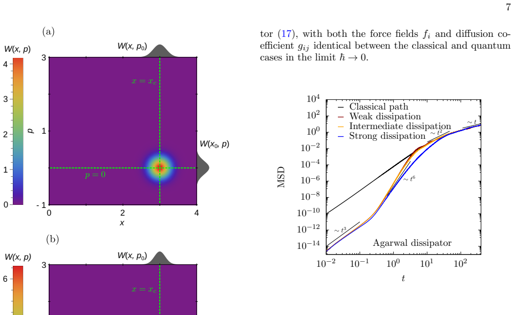
Measure the short-time mean-squared displacement of a harmonically trapped ultracold atom (or trapped ion) whose trap center follows an Ornstein-Uhlenbeck trajectory, at strong dissipation. If the short-time exponent is t^3, the environment behaves like the Agarwal dissipator; if a diffusive regime appears, it behaves like the translated Lindblad dissipator. Alternatively, check whether complete positivity is maintained for non-Gaussian initial states; a violation would rule out Lindblad-type models.
If this is right
- If the translated Lindblad dissipator is the correct model, a quantum active particle can track its moving trap even at strong dissipation while keeping a valid density matrix, opening strongly dissipative quantum-optics realizations.
- If the Agarwal dissipator is the correct model, experiments should observe the classical active-matter short-time scaling (t^3) of the mean squared displacement, with the particle following the trap with an inertial delay.
- The two models give identical steady states for a fixed trap center, so steady-state measurements alone cannot identify the dissipator; time-resolved measurements are essential.
- The short-time mean-squared-displacement exponent is a direct experimental discriminator: a diffusive regime signals a Lindblad-type dissipator, while t^3 scaling signals Agarwal-type friction.
- Because no single dissipator in the considered set satisfies both requirements, any quantum-active-matter experiment must decide which property—positive density matrix or classical limit—is essential for its purpose.
Where Pith is reading between the lines
- An inference the authors do not draw: since the translated Lindblad and Agarwal dissipators share the same steady state for a fixed trap center, any experiment that samples only steady-state spatial distributions cannot tell which dissipator is realized; only time-resolved measurements can.
- I infer that the core trade-off may generalize: for a harmonic trap driven by a stochastic center, any time-local master equation that follows the drive and is completely positive may be forced to deviate from the classical Fokker–Planck structure in the ℏ→0 limit, while any equation that matches the classical structure cannot stay completely positive—a stronger no-go statement worth testing for o
- A testable extension: in a cold-atom realization with a moving optical trap, vary the dissipation strength and measure the short-time mean-squared-displacement exponent; the exponent (diffusive vs t^3) would report which dissipator class the environment actually implements.
- The paper leaves open whether the translated Lindblad dissipator can be derived from an underlying system–bath Hamiltonian; if it cannot, the comparison is between a phenomenological and a microscopic model, and the 'one or the other' conclusion might not apply to physically realizable environments.
Editorial analysis
A structured set of objections, weighed in public.
Referee Report
Summary. The paper studies a single quantum particle confined by a harmonic trap whose center follows an Ornstein-Uhlenbeck trajectory, and compares three time-local master equations for dissipation: a static Lindblad dissipator, a translated Lindblad dissipator whose instantaneous steady state is centered on the moving trap, and the Agarwal (Caldeira-Leggett-type) dissipator. For each model the authors derive a Wigner-function Fokker-Planck equation, compute stationary states for fixed trap center, and evaluate the mean squared displacement numerically at weak, intermediate, and strong dissipation. The central claim is a trade-off: Lindblad-type dissipators preserve complete positivity but do not recover the classical active-OUP dynamics in the classical limit, whereas the Agarwal dissipator supposedly recovers that classical limit but is not CPTP. The paper is clearly written and the comparison is systematic, but the Agarwal branch of this trade-off is not supported by the displayed equations.
Significance. The question addressed is timely for the emerging field of quantum active matter, and the paper offers a useful side-by-side comparison of three dissipator models. The Lindblad Wigner calculations in Appendix B.1 are detailed and reproducible, the stationary solutions (18) and (21) are explicit and plausible, and the numerical MSD comparison across dissipation regimes is informative. If the advertised trade-off were rigorously established, it would give concrete guidance for experiments with moving optical traps. However, as submitted the central claim rests on an algebraic derivation that contains inconsistencies and on a classical-limit statement that is contradicted by the paper's own equations. The paper therefore needs substantial revision before the trade-off can be accepted.
major comments (3)
- [Appendix B.2, Eq. (B25) and Eq. (22)] Using the Moyal product convention adopted in the paper, one has [x,{p,ρ}]_W = 2iℏ(W+p∂_pW). The first term in Eq. (B25) should therefore be (γ/4)(W+p∂_pW), not (ℏγ/4)(W+p∂_pW). In addition, the intermediate results (B18) and (B21) do not agree with a direct Moyal evaluation: (x p ρ)_W contains a +ℏ²/4 ∂²_{xp}W term absent from (B18), and (ρ p x)_W has the opposite sign of the W term from (B21). Thus Eq. (B25) does not follow from its premises and also disagrees with the drift in Eq. (22b). This is load-bearing, not typographical.
- [Section III, Eqs. (17), (22) and the ℏ→0 limit] Even after deleting the spurious ℏ from (B25), Eq. (22) does not reduce to the classical Fokker-Planck equation (17) in the limit ℏ→0. The friction coefficient in Eq. (22b) is γ/4 rather than γ, and the p-diffusion coefficient implied by Eqs. (22a),(22c) is ℏ×γmω/8 coth(ℏω/2k_BT) → γmk_BT/4 (or γk_BT/4 when m=ω=1), not γk_BT. The sentence claiming that 'force fields and diffusion coefficient are identical' is therefore contradicted by the displayed equations. Since this equivalence is the basis for the classical-active branch of the central trade-off, the derivation must be corrected and Fig. 6 with its conclusions re-examined.
- [Section II.B.2, Eq. (11)] The translated Lindblad dissipator is introduced by translating the system operators, but no underlying system-bath Hamiltonian is given. Appendix C only discusses differentiability of x_c(t), not the physical realizability of this time-dependent generator. Because the paper contrasts this model with the Agarwal/Caldeira-Leggett dissipator, the central trade-off is weakened unless the translated Lindblad dissipator is either derived from a microscopic model or explicitly labeled and defended as a phenomenological model.
minor comments (4)
- [Section III, Eqs. (20b), (22b)] After Section II.C the calculations appear to use units with m=ω=1, but this is not stated explicitly. Equations such as (20b) and (22b) contain mω(x−x_c), whereas the classical reference (17b) contains mω²(x−x_c); in dimensionless units with ω=1 these agree, but the manuscript should state this convention.
- [Eqs. (15a), (20a), (22a)] The notation ∂tW = ∂_i(f_iW) + ℏ∂²_{ij}(g_ijW) is ambiguous: it should be made explicit that the actual diffusion coefficient in the Fokker-Planck equation is ℏg_ij, not g_ij.
- [Figures 2, 4, 6] The term 'Dynamic Lindblad dissipator' in the captions is inconsistent with the text's 'translated Lindblad dissipator'; use one name throughout.
- [Appendix B, Eq. (B7)] The star-product expansion is written to O(ℏ³) while the subsequent applications retain only ℏ² terms. This is acceptable but should be stated for clarity.
Circularity Check
No fitted-parameter circularity; only the translated-Lindblad trap-following property is built in by construction. The Agarwal classical-limit derivation has an internal consistency problem, but that is a correctness issue, not circularity.
specific steps
-
self definitional
[Section II.B.2, Eqs. (11)-(12); Section III, Eqs. (20)-(21) and Fig. 4]
"One possible extension of the framework is to modify the dissipator (6) in such a way that the new quantum master equation has its instantaneous steady-state as a Boltzmann state with the harmonic potential centered at x_c(t). ... For this purpose, we consider a dissipator D translated by x_c. This translation is mediated by a translation operator ŽT(x_c) = e^{-ix_c Žp/ħ} ..."
The translated Lindblad dissipator is deliberately constructed by conjugating the static dissipator with the translation operator T(x_c), shifting the creation/annihilation operators to the instantaneous trap position x_c(t). The stationary Wigner solution, which the paper states is 'ensuring that the quantum particle follows the active protocol x_c', is therefore an input of the construction rather than an emergent prediction. This is a self-definitional element for that specific model. However, the MSD scalings, the short-time regimes, and the comparison among dissipators are computed consequences rather than fits, so the circularity is partial and does not by itself invalidate the central comparison.
full rationale
No parameter is fitted to any MSD curve or to the classical Fokker-Planck equation: the static Lindblad dissipator (6), the translated Lindblad dissipator (11), and the Agarwal dissipator (13) are specified independently, and the Wigner-Fokker-Planck equations (15), (20), and (22) are derived from them. The main trade-off, CPTP positivity versus classical-limit behavior, is a comparison of independent model dynamics rather than a reduction of one result to another. The self-citations to Ref. [5] for the t^6 and t^6-t^4 scaling laws and for the sufficiency of 200 trajectories are supporting references; the paper's own simulations exhibit these scalings, so the citations are not load-bearing uniqueness arguments. One minor by-construction element is the translated-Lindblad trap-following property, which is designed into the dissipator and then presented as the behavior of the model. Separately, the claim that the Agarwal Wigner equation (22) reduces exactly to the classical Fokker-Planck equation (17) in the ħ→0 limit is not supported by the displayed algebra: comparing Eq. (B25) with Eq. (22b) shows a factor-of-ħ discrepancy in the drift term, and the resulting friction and diffusion coefficients differ from Eq. (17) by factors of 1/4. This is an internal consistency/correctness issue in the Agarwal branch, not a circularity, but it should be corrected before the classical-limit claim is relied upon.
Axiom & Free-Parameter Ledger
free parameters (2)
- dissipation rates ν+ and ν- =
ν+=1e-8; ν-=1e-2, 1, 10 for weak/intermediate/strong dissipation
- OU process parameters D, τ =
D=0.01, τ=10
axioms (5)
- domain assumption Time-local (Markovian) master equation with the Born-Markov approximation is valid for the driven quantum particle coupled to the bath.
- domain assumption The active drive x_c(t) is a prescribed Ornstein-Uhlenbeck process unaffected by the quantum particle and differentiable in time.
- ad hoc to paper The translated Lindblad dissipator (Eq. 11) represents a legitimate time-local generator for the particle in a moving trap, despite no underlying system-bath Hamiltonian being specified.
- standard math Wigner-Weyl transforms of the dissipators are computed with linear response; higher-order Moyal corrections vanish for the harmonic potential.
- domain assumption Initial state is the ground state of the static harmonic oscillator.
Cite this review
Pith. "Pith review of Modeling dissipation in quantum active matter." pith.science (2026). https://pith.science/paper/BJ7ULUKC
@misc{pith2026251121502,
  author       = {Pith},
  title        = {Pith review of: Modeling dissipation in quantum active matter},
  year         = {2026},
  howpublished = {\url{https://pith.science/paper/BJ7ULUKC}},
  note         = {Machine review of arXiv:2511.21502}
}
read the original abstract
Active matter is characterized by a constant influx and dissipation of energy that gives rise to directed motion. Dissipation requires interactions with an external environment, such that extending the paradigm of active matter to a quantum framework requires an appropriate description of this environment. In this work, we consider a driven quantum particle undergoing noise and dissipation, with external driving exhibiting characteristics of classical activity. We model the non-unitary dynamics with time-local master equations and analyze the particle motion at different time scales for different forms of the master equations, satisfying different criteria. We systematically compare predictions on the dynamics of particle trajectories and thereby we uncover how the particle motion evolves under the interplay of quantum effects, dissipation, and active-like dynamics. These results are essential for guiding possible experiments aimed at realizing quantum analogues of classical active systems.
Figures



Forward citations
Cited by 4 Pith papers
-
Entanglement capacity of complex networks from quantum walks
Source-target entanglement in quantum walks on arbitrary networks is upper-bounded by connectivity, with graph matchings controlling its generation and higher connectivity reducing the maximum in random graphs.
-
Anomalous Mean-Squared Displacement in Quantum Active Matter from a Wigner Phase-Space Framework
Quantum active matter shows mean-squared displacement scaling as t^6 or t^7 derived analytically from a Wigner phase-space master equation.
-
Anomalous Mean-Squared Displacement in Quantum Active Matter from a Wigner Phase-Space Framework
Hybrid Wigner analysis of quantum active matter produces analytical MSD with t^6 (and under specific ICs t^7) scaling for long persistence and large active noise, plus explicit onset times.
-
Phase-dependent role of dissipation across the Aubry-Andr\'e-Harper transition
Bath memory reshapes transport patterns in the extended phase of the AAH transition but mainly renormalizes timescales in the localized phase.
Reference graph
Works this paper leans on
-
[1]
Static Lindblad dissipator We start from the static Lindblad dissipator ˆDL [31], ˆDL ≡ ˆD(ˆρ(t)) = γ 2 ¯n ˆa† ˆρ(t)ˆa−1 2 ˆaˆa†,ˆρ(t) (6) + γ 2 (¯n+ 1) ˆaˆρ(t)ˆa† − 1 2 ˆa†ˆa,ˆρ(t) , where{· · ·,· · · }is an anti-commutator defined byn ˆA, ˆB o = ˆA ˆB+ ˆB ˆA. The annihilation ˆaand creation operators ˆa† are defined as ˆa= r mω 2ℏ ˆx+ i mω ˆp ,(7a) ˆa† ...
-
[2]
This modification would allow the dynamics to properly account for the trap motion on long timescales
Translated Lindblad master equation One possible extension of the framework is to modify the dissipator (6) in such a way that the new quantum master equation has its instantaneous steady-state as a Boltzmann state with the harmonic potential centered atx c(t). This modification would allow the dynamics to properly account for the trap motion on long time...
-
[3]
Agarwal dissipator As an alternative to Lindblad dynamics, we con- sider the Agarwal dissipator [40–43], which in the high- temperature limit recovers the well-known Caldeira- Leggett model [29]. While not strictly CPTP and thus not positivity-preserving, the Agarwal dissipator allows (in contrast to the Lindblad ones) to reproduce the clas- sical Fokker-...
-
[4]
Takasan, K
K. Takasan, K. Adachi, and K. Kawaguchi, Phys. Rev. Res.6, 023096 (2024)
2024
-
[5]
The potential has fixed frequencyωbut the center follows the prescribed Ornstein-Uhlenbeck trajectoryx c(t)
a quantum particle of massmis confined by a time-dependent harmonic potential. The potential has fixed frequencyωbut the center follows the prescribed Ornstein-Uhlenbeck trajectoryx c(t). Thereby, the quan- tum particle is governed by a time-dependent Hamilto- nian of the form ˆH(x c(t)) = ˆp2 2m + 1 2 mω2 (ˆx−xc(t))2 ,(2) wherex c(t) is a classical varia...
-
[6]
Nadolny, C
T. Nadolny, C. Bruder, and M. Brunelli, Phys. Rev. X 15, 011010 (2025)
2025
-
[7]
Adachi, K
K. Adachi, K. Takasan, and K. Kawaguchi, Phys. Rev. Res.4, 013194 (2022)
2022
-
[8]
Khasseh, S
R. Khasseh, S. Wald, R. Moessner, C. A. Weber, and M. Heyl, Phys. Rev. Lett. (2025)
2025
-
[9]
Yamagishi, N
M. Yamagishi, N. Hatano, and H. Obuse, Sci. Rep.14, 28648 (2024)
2024
-
[10]
Elgeti, R
J. Elgeti, R. G. Winkler, and G. Gompper, Rep. Prog. Phys.78, 56601 (2015)
2015
-
[11]
A. P. Antonov, Y. Zheng, B. Liebchen, and H. L¨ owen, Phys. Rev. Res.7, 033008 (2025)
2025
-
[12]
M. Das, C. F. Schmidt, and M. Murrell, Soft Matter16, 7185 (2020)
2020
-
[13]
Penner, L
A.-G. Penner, L. Viotti, R. Fazio, L. Arrachea, and F. von Oppen, Phys. Rev. B112, L180303 (2025)
2025
-
[14]
M. te Vrugt, B. Liebchen, and M. E. Cates, arXiv:2507.21621 (2025)
Pith/arXiv arXiv 2025
-
[15]
Marchetti, J
M. Marchetti, J. Joanny, S. Ramaswamy, T. Liverpool, J. Prost, M. Rao, and R. A. Simha, Rev. Mod. Phys.85, 1143 (2013)
2013
-
[16]
Breuer and F
H.-P. Breuer and F. Petruccione,The theory of open quantum systems(OUP Oxford, 2002)
2002
-
[17]
Bechinger, R
C. Bechinger, R. Di Leonardo, H. L¨ owen, C. Reichhardt, G. Volpe, and G. Volpe, Rev. Mod. Phys.88, 045006 (2016)
2016
-
[18]
Zwanzig, J
R. Zwanzig, J. Chem. Phys.33, 1338 (1960)
1960
-
[19]
Mart ´ ınez-Prat, R
B. Mart ´ ınez-Prat, R. Alert, F. Meng, J. Ign´ es-Mullol, J.-F. Joanny, J. Casademunt, R. Golestanian, and F. Sagu´ es, Phys. Rev. X11, 031065 (2021)
2021
-
[20]
Fodor, R
´E. Fodor, R. L. Jack, and M. E. Cates, Annu. Rev. Con- dens. Matter Phys.13, 215 (2022)
2022
-
[21]
Bebon, J
R. Bebon, J. F. Robinson, and T. Speck, Phys. Rev. X 15, 021050 (2025)
2025
-
[22]
Nathan and M
F. Nathan and M. S. Rudner, Phys. Rev. B102, 115109 (2020)
2020
-
[23]
Nakajima, Progr
S. Nakajima, Progr. Theor. Phys.20, 948 (1958)
1958
-
[24]
M. Stefanini, A. A. Ziolkowska, D. Budker, U. Poschinger, F. Schmidt-Kaler, A. Browaeys, A. Imamoglu, D. Chang, and J. Marino, arXiv:2506.22436 (2025)
Pith/arXiv arXiv 2025
-
[25]
te Vrugt and R
M. te Vrugt and R. Wittkowski, Eur. J. Phys.41, 045101 (2020)
2020
-
[26]
Lindblad, Commun
G. Lindblad, Commun. Math. Phys.48, 119 (1976)
1976
-
[27]
Carmichael,An open systems approach to quantum optics: lectures presented at the Universit´ e Libre de Brux- elles October 28 to November 4, 1991(Springer, 1993)
H. Carmichael,An open systems approach to quantum optics: lectures presented at the Universit´ e Libre de Brux- elles October 28 to November 4, 1991(Springer, 1993)
1991
-
[28]
Hewgill, G
A. Hewgill, G. De Chiara, and A. Imparato, Phys. Rev. Res.3, 013165 (2021)
2021
-
[29]
S. M. Barnett and P. L. Knight, Phys. Rev. A33, 2444 (1986)
1986
-
[30]
B. L. Hu, J. P. Paz, and Y. Zhang, Phys. Rev. D45, 2843 (1992)
1992
-
[31]
Ford and R
G. Ford and R. O’Connell, Physica A243, 377 (1997)
1997
-
[32]
Soret, V
A. Soret, V. Cavina, and M. Esposito, Phys. Rev. A106, 062209 (2022)
2022
-
[33]
S.-Y. Wang, Q. Yang, and F.-L. Zhang, Phys. Rev. E 107, 014108 (2023). 9
2023
-
[34]
Maggi, M
C. Maggi, M. Paoluzzi, N. Pellicciotta, A. Lepore, L. An- gelani, and R. Di Leonardo, Phys. Rev. Lett.113, 238303 (2014)
2014
-
[35]
A. O. Caldeira and A. J. Leggett, Physica A121, 587 (1983)
1983
-
[36]
Y. Fily, J. Chem. Phys.150, 174906 (2019)
2019
-
[37]
Rivas and S
A. Rivas and S. F. Huelga,Open quantum systems, Vol. 10 (Springer, 2012)
2012
-
[38]
De Vega and D
I. De Vega and D. Alonso, Rev. Mod. Phys.89, 015001 (2017)
2017
-
[39]
Szamel, Phys
G. Szamel, Phys. Rev. E90, 012111 (2014)
2014
-
[40]
G. S. Agarwal, Phys. Rev. A2, 2038 (1970)
2038
-
[41]
Caprini and U
L. Caprini and U. M. B. Marconi, Soft Matter14, 9044 (2018)
2018
-
[42]
G. S. Agarwal and S. Chaturvedi, Phys. Rev. E88, 012130 (2013)
2013
-
[43]
Martin, J
D. Martin, J. O’Byrne, M. E. Cates, ´E. Fodor, C. Nar- dini, J. Tailleur, and F. Van Wijland, Phys. Rev. E103, 032607 (2021)
2021
-
[44]
Y.-E. Keta, R. L. Jack, and L. Berthier, Phys. Rev. Lett. 129, 048002 (2022)
2022
-
[45]
Sch¨ uttler, R
J. Sch¨ uttler, R. Garcia-Millan, M. E. Cates, and S. A. M. Loos, Phys. Rev. E112, 024119 (2025)
2025
-
[46]
Wigner, Phys
E. Wigner, Phys. Rev.40, 749 (1932)
1932
-
[47]
G. S. Agarwal, Phys. Rev. A4, 739 (1971)
1971
-
[48]
te Vrugt, G
M. te Vrugt, G. I. T´ oth, and R. Wittkowski, J. Comput. Electron.20, 2209 (2021)
2021
-
[49]
S. Lee, M. Ha, J.-M. Park, and H. Jeong, Phys. Rev. E 101, 022127 (2020)
2020
-
[50]
G. P. Nguyen, R. Wittmann, and H. L¨ owen, J. Phys.: Cond. Mat.34, 035101 (2021)
2021
-
[51]
ACKNOWLEDGEMENTS M.t.V
and dissipative [52] environments will be crucial for bridging the gap between abstract models and experi- mentally accessible setups. ACKNOWLEDGEMENTS M.t.V. is funded by the Deutsche Forschungsgemein- schaft (DFG, German Research Foundation) – SFB 1551, Project-ID 464588647. S.L. thanks R. Kosloff for a dis- cussion on modeling an open quantum system
-
[52]
te Vrugt, Encyclopedia5, 118 (2025)
M. te Vrugt, Encyclopedia5, 118 (2025)
2025
-
[53]
te Vrugt and R
M. te Vrugt and R. Wittkowski, Ann. Phys. (Berlin)532, 2000266 (2020)
2020
-
[54]
Hillery, R
M. Hillery, R. F. O’Connell, M. O. Scully, and E. P. Wigner, Phys. Rep.106, 121 (1984). Appendix A: T ranslation of the quantum dissipators We consider the evolution equation (6) translated by xc, i.e., we apply the translation generator ˆT(x c), ˆT(x c) =e −ixc ˆp/ℏ (A1) to the Hamiltonian ˆH0 ≡ ˆp2 2m + 1 2 mω2 ˆx2,(A2) and the dissipator ˆD. In other w...
1984
-
[55]
Tanimura and P
Y. Tanimura and P. G. Wolynes, Phys. Rev. A43, 4131 (1991)
1991
-
[56]
T. A. Savard, K. M. O’Hara, and J. E. Thomas, Phys. Rev. A56, R1095 (1997)
1997
-
[57]
Beyer and W
M. Beyer and W. Paul, Universe7, 166 (2021)
2021
-
[58]
Briegel and B.-G
H.-J. Briegel and B.-G. Englert, Phys. Rev. A47, 3311 (1993)
1993
-
[59]
Zachos, D
C. Zachos, D. Fairlie, and T. Curtright,Quantum me- chanics in phase space: an overview with selected papers (World Scientific, 2005)
2005
-
[61]
For the Hamiltonian part, the Wigner-Weyl transform is well known [54]
Lindblad dissipator We consider here the creation-annihilation operators in the form ˆ˜a(t) = r mω 2ℏ ˆx−δˆxc(t) + i mω ˆp ,(B1a) ˆ˜a†(t) = r mω 2ℏ ˆx−δˆxc(t)− i mω ˆp ,(B1b) whereδ= 0 for ˆDL (7) andδ= 1 for ˆDT L(12). For the Hamiltonian part, the Wigner-Weyl transform is well known [54]. Here we first show the full expression with the Moyal product; si...
-
[62]
Agarwal dissipator The Wigner-Weyl transform for the Agarwal dissipator is performed analogously by using manipulations performed in Eqs. (B7)-(B8): (ˆxˆpˆρ)W =xpW+ iℏ 2 (W+p∂ pW−x∂ xW) ; (B18) (ˆxˆρˆp)W =xpW+ iℏ 2 (W+p∂ pW+x∂ xW)− ℏ2 4 ∂2 xpW; (B19) (ˆpˆρˆx)W =xpW− iℏ 2 (W+p∂ pW+x∂ xW)− ℏ2 4 ∂2 xpW; (B20) (ˆρˆpˆx)W =xpW+ iℏ 2 (W−p∂ pW+x∂ xW) ; (B21) (ˆxˆ...
-
[101]
The green dashed lines indicate the position (x=x c) of the fixed (p= 0) harmonic potential
The amplitude of the Wigner function values is given by the corresponding color representation; the graphs on the left and right correspond to the peak of the Wigner function at the extremum inxandp, respectively. The green dashed lines indicate the position (x=x c) of the fixed (p= 0) harmonic potential. The dissipation strengthγ= 2(ν − −ν +) (9b) is set...
discussion (0)
Sign in with ORCID, Apple, or X to comment. Anyone can read and Pith papers without signing in.