REVIEW 4 major objections 6 minor 81 references
Drift-Diffusion Matching: Embedding dynamics in latent manifolds of asymmetric neural networks
T0 review · 4 major / 6 minor · reviewed 2026-08-02 · deepseek-v4-flash
Pith's one-line read Drift-diffusion matching makes sufficiently large asymmetric recurrent neural networks embed arbitrary smooth stochastic differential equations in a low-dimensional latent subspace, so that projected network activity reproduces the target d
desk verdict The embedding construction is mathematically clean and the decompositions are genuinely useful, but the paper's headline claim that RNNs can 'faithfully embed arbitrary dynamics' needs quantitative support and a perturbation estimate. read the letter →
The pith
A machine-rendered reading of the paper's core claim, the machinery that carries it, and where it could break.
The reading
What carries the argument
The load-bearing object is the affine latent subspace A={u=Γy+b} combined with the low-rank connectivity parametrization W=ΓW_s, I=ΓI_s+b, B=ΓB_s. This parametrization makes A invariant, giving a one-to-one correspondence between the high-dimensional RNN state and the low-dimensional latent coordinate y. Inside A the latent drift reduces to Eq. (13), a two-layer perceptron that can approximate f(y)+y by universal approximation; noise is matched by B_sB_s^T=σ²I. Two decompositions carry the interpretive weight: a symmetric-asymmetric split of the connectivity (the symmetric part descends an energy landscape in the subspace, the asymmetric part encodes rotation) and a reversible-irreversible s
What would settle it
Train an RNN to embed a standard two-scroll chaotic system using the paper's sampling box, then integrate the trained network autonomously for long times and compare the empirical stationary measure and the maximal expansion rate of nearby trajectories with those of the target system. If the projected dynamics leave the training box, converge to a different attractor, or produce a materially different invariant distribution, the claim that arbitrary smooth stochastic dynamics can be faithfully embedded fails.
Extended reading notes
Core claim
The central claim is that, inside an invariant affine subspace u=Γy+b, the projected drift of the RNN, after moving the 'leak' term -u to the other side, is exactly W_s h(Γy+b)+I_s; hence matching a target SDE dy=f(y)dt+σdw is the same as training a two-layer perceptron to approximate f(y)+y. Because two-layer perceptrons are universal approximators, any sufficiently smooth target drift can in principle be represented. The low-rank parametrization W=ΓW_s, I=ΓI_s+b, B=ΓB_s makes the subspace invariant—trajectories that start inside it never leave—and diffusion is matched by B_sB_s^T=σ²I. The paper demonstrates this for a nonlinear oscillator, two chaotic systems, input-driven switching betwee
Load-bearing premise
The load-bearing premise is that the trained two-layer perceptron approximates f(y)+y well enough, on all regions the stochastic process actually visits, that projected RNN trajectories stay close to the target trajectories over long times—a premise the paper states but does not quantify with any trajectory-level error bound.
Editorial extensions
If this is right
- Any sufficiently smooth target stochastic differential equation—including nonlinear and chaotic systems—can in principle be embedded in an asymmetric low-rank RNN, making such networks universal simulators of latent stochastic dynamics.
- Symmetric connectivity provably confines latent dynamics to generalized gradient flows, so non-gradient computation such as limit cycles, chaos, and directed attractor cycling requires asymmetric connections.
- External inputs can 'tilt' the energy landscape to switch between stored attractors, extending associative memory from initial-state retrieval to input-driven recall.
- Autonomous sequential memory can be built from any gradient system by adding a rotational drift that is divergence-free with respect to the stationary density, producing a nonequilibrium steady state with a preferred order of attractor visits.
- The entropy production rate and the reversible-irreversible decomposition of the latent process carry over exactly to the full network when the noise is elliptic, so nonequilibrium thermodynamics of the circuit can be studied through its low-dimensional manifold.
Reading between the lines
- Editorial inference: because drift-diffusion matching is supervised regression on a bounded sampling box, a natural testable extension is to re-weight the loss by the target's stationary measure or add a smoothness/perturbation penalty; trajectory-level guarantees would then require an explicit bound linking approximation error to pathwise or distributional divergence.
- Editorial inference: the construction provides a converse to neural-manifold analyses—any low-dimensional stochastic dynamics seen in neural data can be realized by an asymmetric low-rank network—so it could serve as a null model for testing whether an empirical manifold is causally computational or merely a projection artifact.
- Editorial inference: the divergence-free rotational currents used for attractor cycling form a general recipe for synthetic nonequilibrium benchmarks; one could embed the same latent process in networks of different sizes and check that measured entropy production stays invariant.
- Editorial inference: the paper reports no clear correlation between structural matrix asymmetry and the entropy production rate of the encoded process, suggesting that irreversible dynamics are encoded jointly in weights, biases, and projection directions; a direct test would be to compare trajectory-level irreversibility measures with several candidate structural asymmetry statistics.
Editorial analysis
A structured set of objections, weighed in public.
Referee Report
Summary. The paper introduces drift-diffusion matching (DDM), a procedure for training low-rank continuous-time RNNs so that a latent affine subspace carries a prescribed target stochastic differential equation dy=f(y)dt+σdw. The central construction is the parameterization W=ΓW_s, I=ΓI_s+b, B=ΓB_s, which makes the affine subspace invariant and reduces the latent drift to a two-layer perceptron: f̂(y)+y = W_s h(Γy+b)+I_s (Eq. 13). Training minimizes a loss (Eq. 14) that matches this perceptron to f(y)+y and matches B_sB_s^T to σ²I. The paper argues from universal approximation that sufficiently large RNNs can faithfully embed arbitrary smooth SDEs, and illustrates the method with stochastic van der Pol, Lorenz, and Dadras systems, as well as input-driven attractor switching and autonomous attractor cycling in nonequilibrium steady states. It also introduces symmetric/asymmetric and reversible/irreversible decompositions of the trained connectivity, and relates latent and network-level entropy production. The invariance proof is mathematically sound; the main gap is the absence of any quantitative link between the regression error minimized in Eq. (14) and the fidelity of the resulting stochastic trajectories over time.
Significance. If the central claim is fully established, the paper offers a clean, constructive method for embedding arbitrary low-dimensional SDEs into high-dimensional RNNs, thereby extending attractor neural network theory beyond symmetric, equilibrium dynamics and connecting it to neural manifold ideas. The invariant-subspace derivation (Eqs. 10–13) is elegant and correct, and the paper contains several genuinely useful explicit constructions: the closed-form optimal symmetric decomposition in App. B, the divergence-free rotational field construction in App. C, the higher-dimensional cycling examples in App. D, and the latent/network equivalence of the entropy production rate in App. E. The paper is not circular: the target vector field appears as a regression target, and the existence of a universal approximator is invoked from an external theorem. However, the strongest advertised claims — that the RNNs 'faithfully embed' arbitrary dynamics and that the numerical examples indeed reproduce the target stochastic processes — are not supported by the present evidence. There is no perturbation estimate translating a small drift error into trajectory or distributional closeness, and the numerica
major comments (4)
- [Sec. II.A, Eqs. (13)–(14)] The load-bearing step is the reduction of the embedding problem to approximating f(y)+y by a two-layer perceptron. Universal approximation guarantees, for any compact K and ε>0, existence of parameters with small sup_K error. But the paper makes no statement about how this approximation error propagates to the stochastic processes. The latent dynamics are exactly the fitted perceptron (because of the low-rank parameterization), so a non-negligible pointwise error directly enters the drift of y(t). To justify 'faithful embedding', the authors need a perturbation estimate linking the regression error in L_DDM to pathwise or distributional closeness of the RNN latent trajectory to the target SDE, including control of what happens when the process leaves the compact training region. For chaotic targets, small drift differences can amplify exponentially; for stochastic targets, the process ca
- [Sec. II.D and Sec. III.B] The numerical validation is qualitative. Figures 2, 3, 6, 9, 10, and 11 show phase portraits and sample neuron traces, but no quantitative comparison between the RNN's latent trajectories and the target SDE. There is no reported test-set drift error, no stationary-density comparison, no autocorrelation or transition-rate comparison, and no code. For the attractor-cycling diffusions, the central phenomenon is the autonomous switching between wells; the paper does not quantify whether the RNN reproduces the switching statistics of the target process. Given that the central claim is about faithful embedding of stochastic dynamics, the numerical section should report quantitative error metrics on held-out data and on trajectory statistics.
- [Sec. IV, Eq. (47)] The HHD decomposition of the network trains two perceptrons with fixed shared first layer (Γ,b) to approximate f_rev and f_irr. The paper correctly notes that fixing the first layer removes the universal-approximation guarantee, but then asserts without evidence that 'this parameterisation is able to approximate the components with very high accuracy'. This is a load-bearing point for the decomposition claims of Sec. IV and Fig. 11. The authors should report the actual residuals of these fits (e.g., L2 error of the learned reversible/irreversible projected fields against the true HHD components) and, ideally, explain why the shared first layer is sufficient for these targets. As it stands, the decomposition is only shown to produce plausible-looking vector fields.
- [App. G and App. H] There is an internal inconsistency in the experimental setup. App. G states that for the deterministic chaotic attractors 'we set λ_diff=0', while App. H says 'Throughout, we train the perceptrons ... We fix λ_diff=20.' The appendix on universal representations and complexity measures therefore rests on an ambiguous or contradictory parameter setting. This needs to be resolved, and the complexity analysis in App. G is exploratory; the lack of any ground-truth validation for the proposed complexity measures should be stated more prominently.
minor comments (6)
- [Eq. (22)] The first component of the Lorenz system is printed as ς(y_2 − y_2); it should be ς(y_2 − y_1).
- [Eq. (14)] The norm in L_DDM is not specified. Please state whether it is an L2 norm, a mean-squared error, or a sup norm, and on what sampling distribution the expectation is taken.
- [Sec. II.A] There is a typo: 'ˆIto's rule' should be 'Itô's rule'.
- [Sec. III.A, App. A.2] The quadratic programming formulation for the tilt vectors is clear, but the choice of the small parameter δ is not discussed; a remark on how δ affects the basin of attraction would be useful.
- [Fig. 4] The PCA reconstruction panel shows the recovered latent coordinates, but the text says the least-squares transformation is applied; it would help to show the residual error of this affine fit.
- [Sec. V and App. D] The paper is commendably explicit about limitations (linear manifold, lack of biological learning rule, autonomous stationary focus, non-smooth non-coplanar example). These limitations should be summarized in the abstract or introduction, since they qualify the 'arbitrary dynamics' claim.
Circularity Check
No circularity: the embedding construction is an honest universal-approximation argument; the trajectory-fidelity gap is a correctness risk, not a circular step.
full rationale
The paper's central existence claim rests on Eq. (13), which is an exact identity inside the invariant affine subspace: under the low-rank parametrisation W=ΓW_s, I=ΓI_s+b, B=ΓB_s, the projected dynamics are dy = (-y + W_s h(Γy+b)+I_s)dt + B_s dw. Thus matching a target SDE, dy=f(y)dt+σdw, reduces to approximating f(y)+y by the two-layer perceptron W_s h(Γy+b)+I_s and matching the diffusion by B_sB_s^T=σ²I_k. This is a constructive reduction to an external theorem (universal approximation, Hornik et al.), not to the paper's own fitted outputs. The DDM loss is an honest regression of f(y)+y and σ²I; no fitted parameter is later renamed as a prediction or used as an axiom. The invariant-subspace and PCA claims are derived in-paper or are standard linear algebra. The symmetric/asymmetric and Helmholtz-Hodge decompositions are motivated and derived inside the paper, not imported from the authors' prior work. Self-citations (Refs. 19, 53, 71) provide background on nonequilibrium brain dynamics, directed-network entropy production, and a supporting NESS calculation; none is load-bearing for the central embedding claim. The main weakness—absence of a quantitative bound linking L_DDM regression error to pathwise or distributional closeness of the RNN and target trajectories over long times—is a correctness risk about how strong the 'faithful embedding' claim is, not circularity. The claim is not forced by definition or by a self-citation chain.
Assumptions & free parameters
free parameters (6)
- λ_diff =
20
- Network size N =
64, 128, 256, 512, 1024
- Training sampling region =
e.g., [-4,4]^2 for VDP; [-25,25]×[-30,30]×[0,50] for Lorenz
- Rotational field parameters α, ξ =
e.g., α=1.5, ξ=0.2 for three-minima; α=2.5, ξ=0.6 for four/five minima
- Gaussian well parameters {a_j, ν_j} and noise σ =
a_j=0.25, ν_j=0.75, σ=0.2 (three-minima)
- Input tilt vectors c_i* =
solved via quadratic programming (App. A2)
assumptions (7)
- standard math Two-layer perceptrons with a nonlinear hidden layer are universal approximators for continuous functions on compact sets (Hornik et al., 1989).
- standard math Itô's formula for the drift of a projected diffusion.
- standard math The Moore-Penrose inverse satisfies Γ†Γ=I_k for full-column-rank Γ.
- domain assumption The target dynamics remain inside the bounded training region for the times considered.
- ad hoc to paper The trained perceptron's regression error is small enough that RNN trajectories stay close to target SDE trajectories.
- ad hoc to paper In the network HHD decomposition, the reversible and irreversible components of the drift can each be represented by a perceptron with the same fixed first layer (Γ,b) and sum to the full trained perceptron.
- domain assumption For EPR equivalence, the diffusion matrix B_s has full row rank (d≥k) and the irreversible force lies in Range(B).
Cite this review
Pith. "Pith review of Drift-Diffusion Matching: Embedding dynamics in latent manifolds of asymmetric neural networks." pith.science (2026). https://pith.science/paper/BJMASSOV
@misc{pith2026260214885,
  author       = {Pith},
  title        = {Pith review of: Drift-Diffusion Matching: Embedding dynamics in latent manifolds of asymmetric neural networks},
  year         = {2026},
  howpublished = {\url{https://pith.science/paper/BJMASSOV}},
  note         = {Machine review of arXiv:2602.14885}
}
read the original abstract
Recurrent neural networks (RNNs) provide a theoretical framework for understanding computation in biological neural circuits, yet classical results, such as Hopfield's model of associative memory, rely on symmetric connectivity that restricts network dynamics to gradient-like flows. In contrast, biological networks support rich time-dependent behaviour facilitated by their asymmetry. Here we introduce a general framework, which we term drift-diffusion matching, for training continuous-time RNNs to represent arbitrary, nonlinear stochastic differential equations (SDEs), with given drift and diffusion coefficients, within a low-dimensional latent subspace. Allowing asymmetric connectivity, we show that RNNs can faithfully embed the drift and diffusion of a given SDE, including nonlinear and nonequilibrium dynamics such as chaotic attractors. As an application, we construct RNN realisations of stochastic systems that transiently explore various attractors through both input-driven switching and autonomous transitions driven by nonequilibrium currents, which we interpret as models of associative and sequential (episodic) memory. To elucidate how these dynamics are encoded in the network, we introduce decompositions of the RNN based on its asymmetric connectivity and its time-irreversibility. Our results extend attractor neural network theory beyond equilibrium, showing that asymmetric neural populations can implement a broad class of dynamical computations within low-dimensional manifolds, unifying ideas from associative memory, nonequilibrium statistical mechanics, and neural computation.
Figures


Figures from the paper (12 more)




Reference graph
Works this paper leans on
-
[1]
Simulating trajectories from SDEs We sample paths from an SDE using theEuler-Maruyama discretisation, xt+∆t =x t +∆t[f(x t )] +∆wt [Σ(xt )],(A1) where∆tis the time-step and∆w t are independent and identi- cally distributed (i.i.d.) multivariate normal random variables with mean zero and covariance∆tI n [66]
-
[2]
III A, we propose an approach for designing an RNN that switches between attractors based on an input
Computing inputs for attractor-switching In Sec. III A, we propose an approach for designing an RNN that switches between attractors based on an input. Here we present the concrete approach used for computingc,G s, andd, in the numerical example. As detailed in Sec. III A, c∈R k makes the local minimumµµµi∗ a global minimum if, c·(µµµi∗ −µµµ j)>V 0 i∗ −V ...
-
[3]
More specifically we use CubicSplinefromscipy.interpolate[68]
Constructing closed curves with splines We compute interpolating closed curves with cubic splines with periodic boundary conditions. More specifically we use CubicSplinefromscipy.interpolate[68]. We then parametrise the curve,γ(t), with 500 time-points and con- struct amatplotlibpath. We can then measure the distance between any point,p, and each discrete...
-
[4]
Panela)of Fig
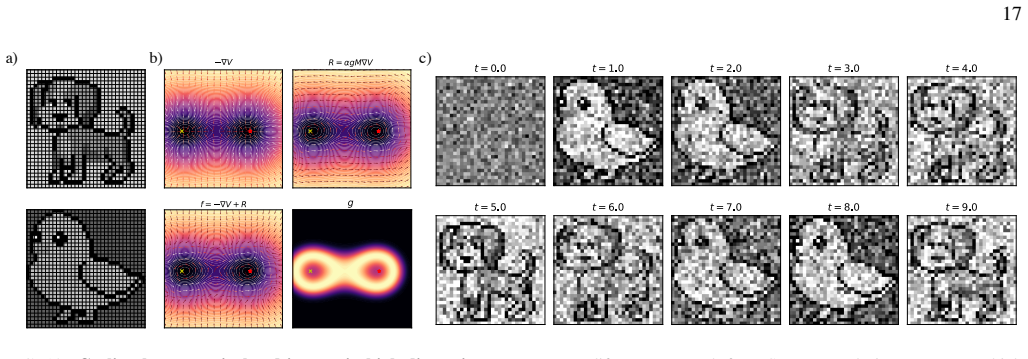
A high-dimensional example with pixel images We consider two grey-scaled, 32×32 images, whose pixel- values are scaled to[0,1]. Panela)of Fig. 12 shows a dog and chick image, respectively. These points can be thought of as pointsµ µµ1,µµµ2 ∈R 1024. We define a Gaussian poten- tial onR 1024 with minima at the points corresponding to the dog and chick image...
-
[5]
As before, we define the attractor dynamics,−∇V, with Gaussian wells
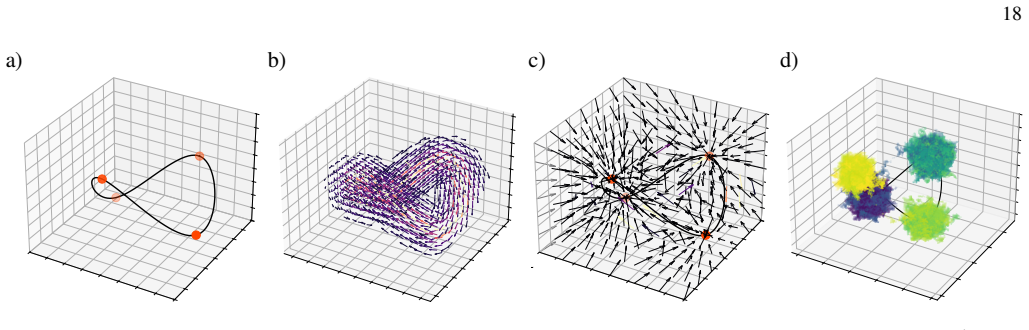
Non-coplanar minima in three dimensions Here we consider a set of minima which are non-coplanar inR 3. As before, we define the attractor dynamics,−∇V, with Gaussian wells. However, the rotational componentR from the coplanar case cannot be applied in this setting. This is because the level sets of the signed distance function are no longer curves, but in...
-
[6]
II, we use the following parameters
Nonlinear systems and RNN representations In Sec. II, we use the following parameters. •Van der Pol.We takeσ=0.25. We train an RNN with N=64, and 25,000 uniform samples from[−4,4] 2 for 30,000 epochs. •Lorenz.We takeσ=0.25. We train an RNN withN= 512, and 125,000 uniform samples from[−25,25]× [−30,30]×[0,50]withλ diff =20 for 100,000 epochs. •Dadras.We ta...
-
[7]
III, we use the following parameters
Switching and cycling attractors In Sec. III, we use the following parameters. •Input-driven switching.We place four minima at (±3,±3)∈R 2, with Gaussian well parameters given bya j =0.125 andν j =1, and noise intensityσ=0.1. We train the RNN withN=256 using 25,000 samples from[−4,4] 2 for 30,000 epochs. Next, we have the three examples of autonomously cy...
2026
-
[8]
D, we use the following parameters
Non-coplanar examples In App. D, we use the following parameters. •Pixel images.We fix minima at the points correspond- ing to the images, with Gaussian wells specified by a j =7,ν j =11. The process hasσ=0.3,ξ=0.5, s=−3.2, andα=40. •Points on the saddle.We place points at the positions given by, µµµ= 0.4 0.7 0.2 1−0.5−0.2 −0.2−0.6 0.4 −0.5 0.2−0.6 ...
Show all 81 references
-
[9]
F, we train RNNs withN=64 with 25,000 samples in[−4,4] 2 for 30,000 epochs and setσ=0.25
Network asymmetry and entropy production In App. F, we train RNNs withN=64 with 25,000 samples in[−4,4] 2 for 30,000 epochs and setσ=0.25
-
[10]
G, we train RNNs withN=1024 with 125,000 samples for 2000 epochs using batches of size 1024
Measuring complexity of chaotic attractors In App. G, we train RNNs withN=1024 with 125,000 samples for 2000 epochs using batches of size 1024. For the Halvorsen attractor, we take the samples in the range [−15,12] 3. For the R ¨ossler attractor, we take[−15,12]× [−15,12]×[0,25]. 22
2000
-
[11]
Decoding the brain: From neural representations to mechanistic models,
M. W. Mathis, A. P. Rotondo, E. F. Chang, A. S. Tolias, and A. Mathis, “Decoding the brain: From neural representations to mechanistic models,”Cell, vol. 187, no. 21, pp. 5814–5832, 2024
2024
-
[12]
Compu- tation through neural population dynamics,
S. Vyas, M. D. Golub, D. Sussillo, and K. V . Shenoy, “Compu- tation through neural population dynamics,”Annual Review of Neuroscience, vol. 43, 2020
2020
-
[13]
Inferring single-trial neural popula- tion dynamics using sequential auto-encoders,
C. Pandarinath, D. J. O’Shea, J. Collins, R. Jozefowicz, S. D. Stavisky, J. C. Kao, E. M. Trautmann, M. T. Kaufman, S. I. Ryu, L. R. Hochberg, J. M. Henderson, K. V . Shenoy, L. F. Abbott, and D. Sussillo, “Inferring single-trial neural popula- tion dynamics using sequential a...
2018
-
[14]
Reconstructing computational system dynamics from neural data with recur- rent neural networks,
D. Durstewitz, G. Koppe, and M. I. Thurm, “Reconstructing computational system dynamics from neural data with recur- rent neural networks,”Nature Reviews Neuroscience, vol. 24, p. 693–710, 2023
2023
-
[15]
Generating coherent patterns of activity from chaotic neural networks,
D. Sussillo and L. F. Abbott, “Generating coherent patterns of activity from chaotic neural networks,”Neuron, vol. 63, no. 4, pp. 544–557, 2009
2009
-
[16]
Optimal control of transient dynamics in balanced networks supports generation of complex movements,
G. Hennequin, T. P. V ogels, and W. Gerstner, “Optimal control of transient dynamics in balanced networks supports generation of complex movements,”Neuron, vol. 82, no. 6, pp. 1394–1406, 2014
2014
-
[17]
Next generation reservoir computing,
D. J. Gauthier, E. Bollt, A. Griffith, and W. A. S. Barbosa, “Next generation reservoir computing,”Nature Communica- tions, vol. 12, no. 5564, 2021
2021
-
[18]
A neural machine code and pro- gramming framework for the reservoir computer,
J. Z. Kim and D. S. Bassett, “A neural machine code and pro- gramming framework for the reservoir computer,”Nature Ma- chine Intelligence, vol. 5, pp. 622–630, 2023
2023
-
[19]
Reservoir- computing based associative memory and itinerancy for com- plex dynamical attractors,
L.-W. Kong, G. A. Brewer, and Y .-C. Lai, “Reservoir- computing based associative memory and itinerancy for com- plex dynamical attractors,”Nature Communications, vol. 15, no. 4840, 2024
2024
-
[20]
Neural networks and physical systems with emer- gent collective computational abilities,
J. Hopfield, “Neural networks and physical systems with emer- gent collective computational abilities,”Proceedings of the Na- tional Academy of Sciences, vol. 79, pp. 2554–2558, 1982
1982
-
[21]
Neurons with graded response have collective computational properties like those of two-state neurons,
J. Hopfield, “Neurons with graded response have collective computational properties like those of two-state neurons,” Proceedings of the National Academy of Sciences, vol. 81, pp. 3088–3092, 1984
1984
-
[22]
Pavliotis,Stochastic Processes and Applications: Diffu- sion Processes, the Fokker-Planck and Langevin Equations
G. Pavliotis,Stochastic Processes and Applications: Diffu- sion Processes, the Fokker-Planck and Langevin Equations. Springer, 2014
2014
-
[23]
D. J. Amit,Modeling Brain Function: The World of Attractor Neural Networks. Cambridge University Press, 1989
1989
-
[24]
Attractor and integrator networks in the brain,
M. Khona and I. R. Fiete, “Attractor and integrator networks in the brain,”Nature Reviews Neuroscience, vol. 23, p. 744–766, 2022
2022
-
[25]
Temporal association in asym- metric neural networks,
H. Sompolinsky and I. Kanter, “Temporal association in asym- metric neural networks,”Physical Review Letters, vol. 57, no. 2861, 1986
1986
-
[26]
Irreversible spin glasses and neural networks,
J. A. Hertz, G. Grinstein, and S. A. Solla, “Irreversible spin glasses and neural networks,” inHeidelberg Colloquium on Glassy Dynamics, Springer, 2006
2006
-
[27]
Dynamics of spin systems with randomly asymmetric bonds: Langevin dynamics and a spherical model,
A. Crisanti and H. Sompolinsky, “Dynamics of spin systems with randomly asymmetric bonds: Langevin dynamics and a spherical model,”Physical Review A, vol. 36, no. 4922, 1987
1987
-
[28]
Nonequilibrium landscape theory of neural networks,
H. Yan, L. Zhao, L. Hu, X. Wang, E. Wang, and J. Wang, “Nonequilibrium landscape theory of neural networks,”Pro- ceedings of the National Academy of Sciences, vol. 100, no. 45, 2013
2013
-
[29]
Nonequilibrium physics of brain dy- namics,
R. Nartallo-Kaluarachchi, M. Kringelbach, G. Deco, R. Lam- biotte, and A. Goriely, “Nonequilibrium physics of brain dy- namics,”Physics Reports, vol. 1152, pp. 1–43, 2026
2026
-
[30]
En- hanced associative memory, classification, and learning with active dynamics,
A. K. Behera, M. Rao, S. Sastry, and S. Vaikuntanathan, “En- hanced associative memory, classification, and learning with active dynamics,”Physical Review X, vol. 13, no. 041043, 2023
2023
-
[31]
Self-orthogonalizing attractor neu- ral networks emerging from the free energy principle,
T. Spisak and K. Friston, “Self-orthogonalizing attractor neu- ral networks emerging from the free energy principle,”arXiv, vol. 2505.22749, 2025
2025 arXiv
-
[32]
Nonequilibrium thermodynamics of associative memory continuous-time recurrent neural net- works,
M. Aguilera, D. D. Martino, I. Garashchuk, and D. Sinelshchikov, “Nonequilibrium thermodynamics of associative memory continuous-time recurrent neural net- works,” inALIFE 2025: Ciphers of Life: Proceedings of the Artificial Life Conference 2025, 2025
2025
-
[33]
Statistical mechanics of recurrent neural networks I—Statics,
A. Coolen, “Statistical mechanics of recurrent neural networks I—Statics,” inHandbook of Biological Physics, vol. 4, pp. 553– 618, Elsevier, 2001
2001
-
[34]
Statistical mechanics of recurrent neural networks II — Dynamics,
A. Coolen, “Statistical mechanics of recurrent neural networks II — Dynamics,” inHandbook of Biological Physics, vol. 4, pp. 619–684, Elsevier, 2001
2001
-
[35]
A neural manifold view of the brain,
M. G. Perich, D. Narain, and J. A. Gallego, “A neural manifold view of the brain,”Nature Neuroscience, vol. 28, p. 1582–1597, 2025
2025
-
[36]
Neu- ral manifolds for the control of movement,
J. A. Gallego, M. G. Perich, L. E. Miller, and S. A. Solla, “Neu- ral manifolds for the control of movement,”Neuron, vol. 94, no. 5, pp. 978–984, 2017
2017
-
[37]
Opening the black box: low- dimensional dynamics in high-dimensional recurrent neural networks,
D. Sussillo and O. Barak, “Opening the black box: low- dimensional dynamics in high-dimensional recurrent neural networks,”Neural Computation, vol. 25, no. 3, pp. 626–649, 2013
2013
-
[38]
Linking connectivity, dy- namics, and computations in low-rank recurrent neural net- works,
F. Mastrogiuseppe and S. Ostojic, “Linking connectivity, dy- namics, and computations in low-rank recurrent neural net- works,”Neuron, vol. 99, no. 3, pp. 609–623, 2018
2018
-
[39]
High-dimensional neuronal activity from low-dimensional latent dynamics: a solvable model,
V . Schmutz, A. Haydaro ˘glu, S. Wang, Y . Feng, M. Caran- dini, and K. D. Harris, “High-dimensional neuronal activity from low-dimensional latent dynamics: a solvable model,” in 39th Conference on Neural Information Processing Systems (NeurIPS 2025), vol. 38, 2025
2025
-
[40]
The low-rank hypothesis of complex systems,
V . Thibeault, A. Allard, and P. Desrosiers, “The low-rank hypothesis of complex systems,”Nature Physics, vol. 20, pp. 294—-302, 2024
2024
-
[41]
Predicting network dynamics without requiring the knowledge of the interaction graph,
B. Prasse and P. V . Mieghem, “Predicting network dynamics without requiring the knowledge of the interaction graph,”Pro- ceedings of the National Academy of Sciences, vol. 119, no. 44, 2022
2022
-
[42]
Testing the mani- fold hypothesis,
C. Fefferman, S. Mitter, and H. Narayanan, “Testing the mani- fold hypothesis,”Journal of the American Mathematical Soci- ety, vol. 29, pp. 983–1049, 2016
2016
-
[43]
Neural manifold analysis of brain circuit dynamics in health and disease,
R. Mitchell-Heggs, S. Prado, G. P. Gava, M. A. Go, and S. R. Schultz, “Neural manifold analysis of brain circuit dynamics in health and disease,”Journal of Computational Neuroscience, vol. 51, pp. 1–21, 2023
2023
-
[44]
Time for memories,
D. V . Buonomano, G. Buzs ´aki, L. Davachi, and A. C. Nobre, “Time for memories,”Journal of Neuroscience, vol. 43, no. 45, pp. 7565–7574, 2023
2023
-
[45]
The ”echo state
H. Jaeger, “The ”echo state” approach to analysing and train- ing recurrent neural networks,” tech. rep., GMD Report 148, German National Research Center for Information Technology, 2001. 23
2001
-
[46]
Eliasmith and C
C. Eliasmith and C. H. Anderson,Neural Engineering: Com- putation, Representation and Dynamics in Neurobiological Sys- tems. MIT Press, 2003
2003
-
[47]
Backpropagation through time: what it does and how to do it,
P. J. Werbos, “Backpropagation through time: what it does and how to do it,”Proceedings of the IEEE, vol. 78, no. 10, pp. 1550–1560, 1990
1990
-
[48]
Learning long-term de- pendencies with gradient descent is difficult,
Y . Bengio, P. Simard, and P. Frasconi, “Learning long-term de- pendencies with gradient descent is difficult,”IEEE Transac- tions on Neural Networks, vol. 5, no. 2, pp. 157–166, 1994
1994
-
[49]
Multilayer feedfor- ward networks are universal approximators,
K. Hornik, M. Stinchcombe, and H. White, “Multilayer feedfor- ward networks are universal approximators,”Neural Networks, vol. 2, no. 5, pp. 359–366, 1989
1989
-
[50]
Goodfellow, Y
I. Goodfellow, Y . Bengio, and A. Courville,Deep Learning. MIT Press, 2016
2016
-
[51]
Helmholtz decomposition and po- tential functions for n-dimensional analytic vector fields,
E. Gl ¨otzl and O. Richters, “Helmholtz decomposition and po- tential functions for n-dimensional analytic vector fields,”Jour- nal of Mathematical Analysis and Applications, vol. 525, no. 2, p. 127138, 2023
2023
-
[52]
The entropy production of stationary diffusions,
L. D. Costa and G. A. Pavliotis, “The entropy production of stationary diffusions,”Journal of Physics A: Mathematical and Theoretical, vol. 56, no. 36, p. 365001, 2023
2023
-
[53]
Non-reversible processes: GENERIC, hypocoercivity and fluctuations,
M. H. Duong and M. Ottobre, “Non-reversible processes: GENERIC, hypocoercivity and fluctuations,”Nonlinearity, vol. 36, no. 1617, 2023
2023
-
[54]
J. C. Sprott,Elegant Chaos: Algebraically Simple Chaotic Flows. World Scientific, 2010
2010
-
[55]
A novel three-dimensional au- tonomous chaotic system generating two, three and four-scroll attractors,
S. Dadras and H. R. Momeni, “A novel three-dimensional au- tonomous chaotic system generating two, three and four-scroll attractors,”Physics Letters A, vol. 373, pp. 3637–3642, 2009
2009
-
[56]
LIII. On lines and planes of closest fit to sys- tems of points in space,
K. Pearson, “LIII. On lines and planes of closest fit to sys- tems of points in space,”The London, Edinburgh, and Dublin Philosophical Magazine and Journal of Science, vol. 2, no. 11, pp. 559–572, 1901
1901
-
[57]
Neu- ral population dynamics during reaching,
M. M. Churchland, J. P. Cunningham, M. T. Kaufman, J. D. Foster, P. Nuyujukian, S. I. Ryu, and K. V . Shenoy, “Neu- ral population dynamics during reaching,”Nature, vol. 487, p. 51–56, 2012
2012
-
[58]
Dimensionality reduction for large-scale neural recordings,
J. P. Cunningham and B. M. Yu, “Dimensionality reduction for large-scale neural recordings,”Nature Neuroscience, vol. 17, p. 1500–1509, 2014
2014
-
[59]
Recurrent neural network models for working memory of continuous vari- ables: activity manifolds, connectivity patterns, and dynamic codes,
C. J. Cueva, A. Ardalan, M. Tsodyks, and N. Qian, “Recurrent neural network models for working memory of continuous vari- ables: activity manifolds, connectivity patterns, and dynamic codes,”arXiv, vol. 2111.01275, 2021
2021 arXiv
-
[60]
Vidal, Y
R. Vidal, Y . Ma, and S. S. Sastry,Generalized Principal Com- ponent Analysis. Springer, 2016
2016
-
[61]
Free energy, value, and attractors,
K. Friston and P. Ao, “Free energy, value, and attractors,”Com- putational and Mathematical Methods in Medicine, vol. 2012, no. 937860, 2011
2012
-
[62]
Energy-based models,
Y . LeCun, S. Chopra, R. Hadsell, M. Ranzato, and F. J. Huang, “Energy-based models,” inPredicting Structured Data, MIT Press, 2007
2007
-
[63]
Broken detailed balance and entropy production in directed networks,
R. Nartallo-Kaluarachchi, M. Asllani, G. Deco, M. L. Kringel- bach, A. Goriely, and R. Lambiotte, “Broken detailed balance and entropy production in directed networks,”Physical Review E, vol. 110, no. 034313, 2024
2024
-
[64]
Non- reciprocal phase transitions,
M. Fruchart, R. Hanai, P. B. Littlewood, and V . Vitelli, “Non- reciprocal phase transitions,”Nature, vol. 592, pp. 363–369, 2021
2021
-
[65]
Curl descent: Non-gradient learning dynamics with sign-diverse plasticity,
H. Ninou, J. Kadmon, and N. A. Cayco-Gajic, “Curl descent: Non-gradient learning dynamics with sign-diverse plasticity,” in39th Conference on Neural Information Processing Systems (NeurIPS 2025)., 2025
2025
-
[66]
Jiang, M
D.-Q. Jiang, M. Qian, and M.-P. Qian,Mathematical Theory of Nonequilibrium Steady States: On the Frontier of Probability and Dynamical Systems. Springer, 2004
2004
-
[67]
V . I. Bogachev,Measure Theory. Springer, 2007
2007
-
[68]
Engineering recurrent neural networks from task-relevant manifolds and dynamics,
E. Pollock and M. Jazayeri, “Engineering recurrent neural networks from task-relevant manifolds and dynamics,”PLOS Computational Biology, vol. 16, no. 8, p. e1008128, 2020
2020
-
[69]
Theory of orientation tuning in visual cortex,
R. B. Yishai, R. L. Bar-Or, and H. Sompolinsky, “Theory of orientation tuning in visual cortex,”Proceedings of the National Academy of Sciences, vol. 92, pp. 3844–3848, 1995
1995
-
[70]
Shaping manifolds in equivariant recurrent neural networks,
A. D. Bernardo, A. Valente, F. Mastrogiuseppe, and S. Ostojic, “Shaping manifolds in equivariant recurrent neural networks,” arXiv, vol. 2511.04802v2, 2025
2025
-
[71]
Recurrent network models of sequence generation and memory,
K. Rajan, C. D. Harvey, and D. W. Tank, “Recurrent network models of sequence generation and memory,”Neuron, vol. 90, no. 1, pp. 128–142, 2016
2016
-
[72]
Nonequilibrium thermodynamics of the asymmetric Sherrington-Kirkpatrick model,
M. Aguilera, M. Igarashi, and H. Shimazaki, “Nonequilibrium thermodynamics of the asymmetric Sherrington-Kirkpatrick model,”Nature Communications, vol. 14, no. 3685, 2023
2023
-
[73]
A unifying framework for mean-field theories of asymmetric kinetic Ising systems,
M. Aguilera, S. A. Moosavi, and H. Shimazaki, “A unifying framework for mean-field theories of asymmetric kinetic Ising systems,”Nature Communications, vol. 58, 2021
2021
-
[74]
Decomposing the local arrow of time in interacting systems,
C. W. Lynn, C. M. Holmes, W. Bialek, and D. J. Schwab, “Decomposing the local arrow of time in interacting systems,” Physical Review Letters, vol. 129, no. 118101, 2022
2022
-
[75]
A complete recipe for stochastic gradient MCMC,
Y .-A. Ma, T. Chen, and E. B. Fox, “A complete recipe for stochastic gradient MCMC,” inNIPS’15: Proceedings of the 29th International Conference on Neural Information Process- ing Systems, vol. 2, pp. 2917 – 2925, 2015
2015
-
[76]
Kloeden and E
P. Kloeden and E. Platen,Numerical Solution of Stochastic Dif- ferential Equations. Springer, 1992
1992
-
[77]
Hastie, R
T. Hastie, R. Tibshirani, and J. Friedman,The Elements of Statistical Learning: Data Mining, Inference, and Prediction. Springer, 2009
2009
-
[78]
Scipy 1.0: fundamental algorithms for scientific comput- ing in Python,
P. Virtanen, R. Gommers, T. E. Oliphant, M. Haber- land, T. Reddy, D. Cournapeau, E. Burovski, P. Peterson, W. Weckesser, J. Bright, S. J. van der Walt, M. Brett, J. Wil- son, K. J. Millman, N. Mayorov, A. R. J. Nelson, E. Jones, R. Kern, E. Larson, C. J. Carey, ˙Ilhan Polat, ...
2020
-
[79]
M. P. do Carmo,Differentiable Geometry of Curves and Sur- faces. Prentice-Hall, 1976
1976
-
[80]
J. M. Lee,Introduction to Smooth Manifolds. Springer, 2000
2000
-
[81]
Coarse-graining nonequilibrium diffusions with Markov chains,
R. Nartallo-Kaluarachchi, R. Lambiotte, and A. Goriely, “Coarse-graining nonequilibrium diffusions with Markov chains,”arXiv, vol. 2511.05366, 2025
2025 arXiv
Reviewed August 2, 2026 · model on record in the stance chip above.
Discussion (0). Continue with ORCID to comment.