Imaging through rough interfaces: The shower curtain effect

Cristophe Gomez (I2M); Knut S{\o}lna

REVIEW 2 major objections 4 minor 20 references

Imaging through a rough interface is governed by a single blurring length, βint, that grows linearly with distance from the object to the interface.

Reviewed by Pith at T0; open to challenge. T0 means a machine referee read the full paper against a public rubric. the ladder, T0–T4 →

Challenge this review Re-run · record.json Download PDF Read on arXiv ↗

T0 review · deepseek-v4-flash

2026-08-01 13:48 UTC pith:BPIUQY7G

load-bearing objection The second-order imaging theory and the βint parameter are solid and worth reading; the optical SNR section rests on an invalid fourth-order moment in Appendix D and should not be trusted as-is. the 2 major comments →

arxiv 2607.18947 v1 pith:BPIUQY7G submitted 2026-07-21 math-ph math.MPphysics.class-ph

Imaging through rough interfaces: The shower curtain effect

Cristophe Gomez (I2M) , Knut S{\o}lna This is my paper

classification math-ph math.MPphysics.class-ph MSC 35Q6078A45

keywords shower curtain effectrough interface scatteringspeckle statisticsparaxial wave propagationmatched field imagingoptical imaging resolutionsignal-to-noise ratiorandom phase screen

verification ladder T0 review T1 audit T2 compute T3 formal T4 reserved

The pith

A machine-rendered reading of the paper's core claim, the machinery that carries it, and where it could break.

This paper claims that imaging through a randomly rough interface — the setting behind the shower curtain effect — is controlled by one parameter: βint = zint |1 − c0/c1| √D. Here zint is the distance from the object to the interface, c0 and c1 are the wave speeds on either side, and D is the mean-square slope of the interface fluctuations. In the critical scaling, where the interface correlation length matches the beam width, and in the strong-scattering limit, the mean optical image becomes the ideal image blurred by a Gaussian of width βint, and the signal-to-noise ratio depends only on βint. The same parameter sets the width of the speckle fluctuations in matched-field imaging. If the paper is right, the shower curtain effect is fundamentally a propagation phenomenon: blur and image fluctuations grow linearly as the scattering layer is moved away from the object, and they vanish when the interface is flat.

Core claim

For a monochromatic paraxial source imaged through a single rough interface separating two homogeneous media, the paper derives a reduced observation model in which all random scattering enters through the operator Kε(τ,k,k′) = (2π)^(−2)∫ e^{i(k′−k)·x} e^{iτV(x/ε^{γ−1/2})} dx. In the critical regime γ=1/2 with strong scattering, the fourth-order statistics of this operator converge to a universal form that depends on the interface only through D, the curvature of its covariance at zero. As a consequence, the mean optical image is the ideal image convolved with a Gaussian kernel of width βint, and images at different frequencies fluctuate as if a single Gaussian random displacement were appli

What carries the argument

The load-bearing object is the interface scattering operator Kε(τ,k,k′), which maps a transverse Fourier mode k′ to k with random phase τV(x/ε^{γ−1/2}); the value τ = ωo|s0−s1| fixes the medium contrast. The critical step is the evaluation of the fourth moment of Kε in the strong-scattering limit using the local quadratic expansion of the covariance, C(x) ≈ C(0) − D|x|²/2, for a Gaussian V. This yields a universal Gaussian factor exp(−|Δ|²/(2τ²D))/(2πτ²D) with momentum-conserving delta functions, which in turn produces the Gaussian blur kernel of width βint and the representation of all image fluctuations by one effective Gaussian displacement X. The same kernel κ(Δk,k) already controls the

Load-bearing premise

The Gaussian blur formula and especially the SNR and covariance results assume the interface fluctuations are Gaussian and that their covariance is locally quadratic at the scattering scale; that quadratic-Gaussian condition is stated in Appendix D and is not guaranteed by the paper's general Assumption 1.

What would settle it

Take a point-like or chartered source, a rough interface with known D, and vary the object–interface distance zint while recording the image width and the covariance of images at two colors. If the blur width does not grow as zint|1−c0/c1|√D, or if the two-color covariance is not equivalent to a single Gaussian displacement (for instance, if frequency diversity decorrelates the fluctuations), the central claim fails. A targeted version uses a non-Gaussian rough surface with the same D: the mean image should still be Gaussian-blurred, but the SNR should deviate from the paper's formula.

Watch this falsifier — get emailed when new claim-graph text bears on it.

If this is right

Image blur grows linearly with object–interface distance: βint = zint |1−c0/c1| √D, so placing the scattering layer close to the object restores resolution while leaving the layer itself unchanged.
In the strong-scattering critical regime the image statistics become frequency-independent and universal; neither multifrequency averaging nor local spatial smoothing reduces the fluctuations because a single random Gaussian displacement drives them.
Optical intensity-only imaging is far more robust than matched-field imaging: random phase distortions barely affect intensity, so the dominant effect is the βint blur rather than phase noise.
In the rapidly varying interface regime the image shape is preserved but contrast is reduced by |φV(Δk)|², while in the slowly varying regime the image approaches the flat-interface result; only the critical regime produces simultaneous blur and fluctuations.

Where Pith is reading between the lines

These are editorial extensions of the paper, not claims the author makes directly.

The universality suggests a simple calibration strategy: measure the blur at one object distance and one contrast, extract D, and predict resolution and SNR at any other geometry without knowing the full interface spectrum.
The same fourth-moment machinery should extend to stacked rough interfaces; if the βint contributions add in quadrature, a multilayer curtain would behave like one effective rough interface, which could be tested numerically.
Because the randomness is effectively one-dimensional (a common displacement X), methods that scan frequency or detector position will not decorrelate the noise; only changing the interface realization itself—moving the curtain—can average it out.
The mean Gaussian blur may survive for non-Gaussian interface fluctuations, but the SNR formula and the conclusion about averaging should not; an experiment comparing Gaussian and engineered non-Gaussian surfaces would separate the robust geometric part from the model-dependent part.

Editorial analysis

A structured set of objections, weighed in public.

Desk editor's note, referee report, simulated authors' rebuttal, and a circularity audit.

Desk Editor's Note

The second-order imaging theory and the βint parameter are solid and worth reading; the optical SNR section rests on an invalid fourth-order moment in Appendix D and should not be trusted as-is.

read the letter

Colleague,

Read this for the βint result and the matched-field analysis; ignore the optical SNR claims until the fourth-order moment is redone.

What's new: the rough-interface formulation of the shower curtain effect is a genuine departure from the volumetric random-medium treatments, and the explicit formulas for resolution and variance in the critical scaling γ=1/2 are useful. I particularly like the clean statement that blur and matched-field fluctuation support are controlled by βint=zint|1−c0/c1|√D, and the flat-interface and fast-fluctuation limits behave correctly. The derivations of Proposition 3.2 and the mean optical image (Proposition 4.1) are careful and self-contained; Appendix C gives a reasonable Laplace argument for the second moment.

Now the soft spots, in order of importance.

The load-bearing problem is Appendix D. The fourth-order moment is computed by replacing Var(V(0)−V(y1)−aV(y2)+aV(y3)) with D|y1+a(y2−y3)|². That quadratic form is the correct local approximation at the origin, but it is applied as if it were global. In reality the phase combination is exactly zero on the manifold y1=0, y2=y3 for every R, not just near zero. Near that manifold, with R outside the correlation length, the leading variance is D|y1|²+a²D|y2−y3|², no cross term. The change of variables in the proof then misses that continuum and fabricates an additional delta. The upshot is that equation (45) is not established; Proposition 4.3 and the SNR formula (49) are unsupported. The 'single Gaussian displacement' interpretation and the claim that frequency/position averaging cannot reduce variance are direct consequences of that faulty step. The Gaussian assumption isn't the problem—the error survives for Gaussian V.

Minor but real: eq. (14) states 2s0/(s0+s1)=2c0/(c0+c1), but Appendix B correctly gives 2c1/(c0+c1). Looks like a typo, but it should be fixed. Also, the experimental comparison fits α in βint=αzint rather than measuring D and contrast independently; calling that 'direct evidence' is generous.

Bottom line: the second-order theory is a solid contribution and the paper is worth a serious referee. The optical SNR section needs a corrected fourth-order computation or the claims should be retracted. I'd send it to review, with a referee who will actually check Appendix D.

Referee Report

2 major / 4 minor

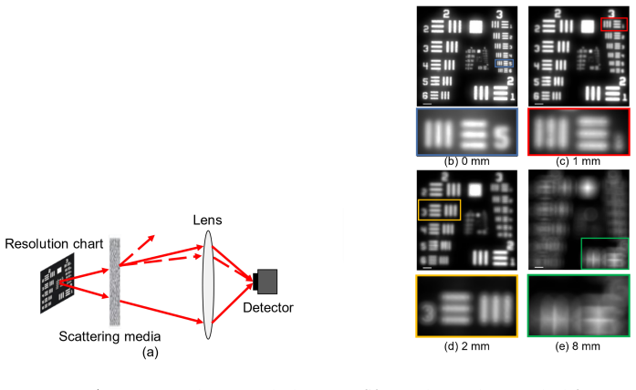
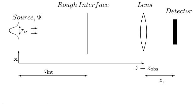
Summary. The manuscript develops an asymptotic theory of passive imaging through a single random rough interface in the paraxial, high-frequency regime. The source is a localized beam; the interface is modeled as a stationary random surface with amplitude σ and correlation length l_c, parameterized by a scaling exponent γ. The authors derive the transmitted field in terms of a random scattering operator, then analyze matched-field and optical imaging. In the critical scaling γ=1/2 and the strong-scattering regime, they claim that the optical image is the ideal image blurred by a Gaussian kernel of width β_int = z_int |1−c0/c1| √D, and that the image covariance is universal and driven by a single effective Gaussian displacement, so that frequency/position averaging is ineffective. A comparison with a published USAF-chart experiment shows approximately linear growth of the blur with source–interface separation.

Significance. If the fourth-order claims are correct, the paper would provide a rare tractable rough-interface model for the shower-curtain effect, with explicit formulas for resolution and SNR and a single dimensionless parameter β_int/ℓ_Ψ. The second-order matched-field and optical mean-image derivations are self-contained and have useful internal checks (flat-interface limit, the three γ-regimes). The manuscript also makes a concrete, falsifiable prediction—linear scaling of the blur with z_int—and connects it to data. However, the fourth-order statistical foundation is not sound in its current form, and the central 'universal Gaussian covariance' claim depends on that foundation.

major comments (2)

[Appendix D, eqs. (D1)–(D3) and Proposition 4.2] The proof of the fourth-order moment is invalid. For S = V(0) − V(y1) − aV(y2) + aV(y3), on the noncompact manifold y1 = 0, y2 = y3 = R, S ≡ 0 for every R, so the characteristic function is identically 1 there. Near this manifold with |R| large, Var(S) ≈ D|y1|^2 + a^2 D|y2−y3|^2, not D|y1 + a(y2−y3)|^2; the cross term in the latter is absent when y2,y3 are outside the correlation length of the origin. Replacing the covariance by its local quadratic expansion for all y1,y2,y3 in (D3), then integrating over u = y2, v = y3, produces the extra delta δ(a(k′−k) − (k̃′−k̃)) in (45) and suppresses a separate Gaussian factor in the second momentum transfer. This is not a Gaussianity issue: the same failure occurs for Gaussian V with finite correlation length. Since Proposition 4.3’s covariance formula, Eqs. (47)–(48), and the SNR conclusions in Eq. (49) and Discussion 4.2 are direct consequences
[Appendix D, Proposition D.1 vs §4.1] Proposition D.1 is stated for V satisfying only Assumption 1, but the proof uses Gaussianity at the step leading to (D3) ('as the interface fluctuations V are assumed to be Gaussian'). The Gaussian assumption is introduced informally in the text of §4.1, and the introduction claims that fourth-order statistics are computed 'without requiring a Gaussian approximation.' This is internally inconsistent. If the fourth-moment result is intended only for Gaussian V, the proposition statement, the text, and the abstract-level claims of universality must be revised accordingly.

minor comments (4)

[Eq. (14)] The displayed identity T = 2s0/(s0+s1) = 2c0/(c0+c1) is algebraically false: with s_j = 1/c_j, one has 2s0/(s0+s1) = 2c1/(c0+c1), as correctly used in Appendix B. Please correct the displayed equality.
[Example 1.1 Revisited and Figure 5] The linear fit α = 0.1 is used without error bars or a goodness-of-fit measure. The comparison is acceptable as an illustration, but the text should not describe it as 'direct evidence' without at least a rough quantitative assessment of the fit uncertainty.
[Proof of Proposition 4.3, §4.1] The proof is only an outline; after applying Proposition 4.2, the text says 'then we can conclude in a similar fashion' and does not display the intermediate reduction. Given that the result is central, a fuller derivation (or a reference to a complete appendix) is needed.
[Appendix D, notation] The curvature parameter D is defined in Remark 3.1 as −C″(0) and in Appendix D as −ρ″(0) σ_V^2/ℓ_V^2. These are consistent under the Gaussian model, but the notation should be harmonized to avoid confusion.

Circularity Check

0 steps flagged

Central derivation is self-contained; no circular reduction found. Only minor self-citations and a fitted experimental comparison appear, neither of which is load-bearing.

full rationale

The paper's main derivation chain is not circular. It starts from the wave equation and the rough-interface model, derives the effective scattering operator Kε (Appendix B), then computes second-order moments (Propositions 3.1, 3.2, 4.1) and a fourth-order moment (Appendix D) under explicit asymptotic assumptions. The Gaussian blurring kernel in (46) is obtained by a Laplace-type asymptotic evaluation of the covariance curvature parameter D, not by inserting the claimed blur as an input. βint is a derived combination of zint, contrast, and D; its reappearance in (46) and (49) is a consequence of the calculation, not a definitional tautology. The flat-interface limits (ϕV ≡ 1, κ(τ,k)=δ(k), βint=0) provide internal consistency checks. Reference [8] is by the same authors, but the paper reproduces the main steps in Appendices A.2 and B, so the self-citation is methodological rather than load-bearing. The experimental comparison in Section 4.2 uses a fitted slope α = 0.1 for βint = αzint; this is a consistency check with one free parameter, not a parameter-free confirmation, but it is ancillary and does not enter the derivation of the imaging formulas. The possible mathematical flaw in Appendix D, and the discrepancy between Proposition D.1's statement (Assumption 1 only) and the Gaussian assumption used in its proof, are correctness risks, not circularity.

Axiom & Free-Parameter Ledger

2 free parameters · 7 axioms · 0 invented entities

The core theory is parameter-free beyond physical inputs (zint, c0/c1, D); the only fitted constant is the experimental slope α=0.1, which absorbs D and the contrast for the USAF-chart comparison. The main unproven inputs are the smooth-interface phase-screen approximation from [8], the Gaussian assumption used for fourth-order speckle statistics, and the strong-scattering/local-curvature limit.

free parameters (2)

experimental slope α = 0.1 (blur in mm per source separation in mm)
In Example 1.1 Revisited, the linear model βint=αzint is fit to roughly estimated blur widths (Figure 5). α absorbs the unknown interface curvature D and speed contrast |1−c0/c1|, so this is a fitted parameter, not an independent prediction.
scaling constant γ* in Appendix C = O(1), unspecified
Introduced in eq. (C1) to balance ℓVℓΨω0/(c0zint) with σVΔk. Its value is not fixed by the theory, but it cancels in the final expression for βint.

axioms (7)

domain assumption Interface random field V is mean-zero, stationary, isotropic, bounded, rapidly mixing, smooth, with bounded second derivatives (Assumption 1).
Controls all statistical limits and the validity of the asymptotic expansions; not derived from physics.
domain assumption Source profile Ψ is smooth and rapidly decaying (Assumption 2).
Needed for Fourier transforms and the asymptotic error estimates.
domain assumption High-frequency paraxial scaling with ε≪1, r0∼√εL0, σ∼λ, and lc∼r0 in the critical regime γ=1/2.
The entire analysis is restricted to this separation-of-scales regime; results do not apply outside it.
domain assumption Field and normal derivative are continuous across the rough interface (eq. 13); no shadowing or multiple-scattering at the interface.
Justified for a smooth interface in Appendix A.2, but neglects slope/shadowing effects that could matter at roughness amplitude σ∼λ.
domain assumption The transmitted field across the interface is, at leading order, the incident field times T e^{iωo(s0−s1)Δz(x)} (Appendix B, eq. B5): a pure random phase-screen model.
This is the load-bearing effective interface model, imported from the authors' prior framework [8]; all subsequent imaging formulas depend on it.
domain assumption V is Gaussian for the fourth-order moment and explicit examples (Section 4.1, Prop. 4.2; Appendix D).
Stronger than Assumption 1; required for the universal Gaussian covariance and the SNR formula (49).
standard math Strong-scattering regime |σVΔk|≫1 and Laplace approximation with local quadratic expansion of the covariance (eq. 38, Appendix C).
Standard asymptotic technique; the local quadratic expansion of ρV is a Taylor expansion under Assumption 1.

pith-pipeline@v1.3.0-alltime-deepseek · 24283 in / 13967 out tokens · 127684 ms · 2026-08-01T13:48:21.120014+00:00 · methodology

0 comments

read the original abstract

The quality of an image observed through a scattering layer, such as a shower curtain, depends strongly on the relative position of the scattering layer between the object and the observer. This well-known phenomenon is commonly referred to as the shower curtain effect. When the scattering layer is placed close to the observer, the image is strongly degraded, whereas if it is located close to the object, the object may still be observed with relatively high resolution. Previous analyses of the shower curtain effect have primarily modeled the scattering layer as a section of a random medium. In this work, we present a new analysis in which the scattering layer is modeled instead as a rough interface, a description that arises naturally in many physical configurations. Within this framework, we derive explicit characterizations of both the image resolution and the signal-to-noise ratio, and determine how these quantities depend on the statistical properties of the rough interface and on its relative location between the object and the observer.

Figures

Figures reproduced from arXiv: 2607.18947 by Cristophe Gomez (I2M), Knut S{\o}lna.

**Figure 1.** Figure 1: Figure a): Experimental setup with the 1951 USAF resolution chart on the left, a ground-glass scattering layer in the middle, and a detector with an imaging lens on the right. The wave field transmitted through the resolution chart is scattered by the ground glass before reaching the detector. The detector and the resolution chart satisfy a conjugate imaging relationship. Figure b)–e) Images recorded for d… view at source ↗

**Figure 2.** Figure 2: Source imaging through a random rough interface. The source is located on the left and the detector on the right. We assume that both the interface location zint and the observation distance zobs are of order L0. We consider a high-frequency regime ε := c0 L0ωo = λ0 2πL0 ≪ 1, together with a paraxial scaling characterized by r 2 0 λ0 ∼ L0. (3) Equivalently, the Rayleigh length LR = πr2 0 λ0 is comparable t… view at source ↗

**Figure 3.** Figure 3: Source imaging in the optical set-up. The detector is a camera or photodetector that records the wave intensity. The source plane z = 0 and the detector plane z = zint + zi are conjugate, i.e. the focal length L of the lens located in the plane z = zobs satisfies (40). which accounts for the different propagation speeds on either side of the interface. The detector plane is chosen to be conjugate to the so… view at source ↗

**Figure 4.** Figure 4: Signal-to-noise ratio (49) as a function of the relative blurring parameter η = βint/ℓΨ and the normalized image offset ρ. Increasing η corresponds to stronger shower-curtain blurring and reduces the image stability. The observed trend is consistent with the theoretical prediction. Most importantly, the figure illustrates the essential geometric nature of the shower-curtain effect: the farther the object i… view at source ↗

**Figure 5.** Figure 5 [PITH_FULL_IMAGE:figures/full_fig_p028_5.png] view at source ↗

discussion (0)

Reference graph

Works this paper leans on

20 extracted references

[1]

Acoustic scattering models from rough surfaces: A brief review and recent advances

Darmon M, Dorval V, Baqu´ e F. Acoustic scattering models from rough surfaces: A brief review and recent advances. Applied Sciences. 2020;10:8305

2020
[2]

Experimental investigation of the inﬂuence of the relative position of the scattering layer on image quality: The shower curtain eﬀect

Dror I, Sandrov A, Kopeika NS. Experimental investigation of the inﬂuence of the relative position of the scattering layer on image quality: The shower curtain eﬀect. Applied Optics. 1998;37:6495–6499

1998
[3]

Optical imaging through dynamic turbid media using the Fourier-domain shower-curtain eﬀect

Edrei E, Scarcell, G. Optical imaging through dynamic turbid media using the Fourier-domain shower-curtain eﬀect. Optica. 2016;3:71–74

2016
[4]

A critical survey of approximate scattering wave the- ories from random rough surfaces

Elfouhaily TM, Gu´ erin CA. A critical survey of approximate scattering wave the- ories from random rough surfaces. Waves in Random Media. 2004;14:R1–R40

2004
[5]

Wave Propagation and Time Reversal in Randomly Layered Media

Fouque, JP, Garnier J, Papanicolaou G, Sølna K. Wave Propagation and Time Reversal in Randomly Layered Media. Springer, New York; 2007

2007
[6]

Light scattering by periodic rough sur- faces: Equivalent jump conditions

Gallas B, Maurel A, Marigo JJ, Ourir A. Light scattering by periodic rough sur- faces: Equivalent jump conditions. Journal of the Optical Society of America A. 2017;34:2181–2188

2017
[7]

Shower curtain eﬀect and source imaging

Garnier J, Sølna K. Shower curtain eﬀect and source imaging. Inverse Problems and Imaging. 2024;18:993–1023

2024
[8]

Generalized Snell’s laws for rough interfaces

Gomez C, Sølna K. Generalized Snell’s laws for rough interfaces. 2026;arXiv:2603.17488. 29

arXiv 2026
[9]

Wave Propagation and Scattering in Random Media

Ishimaru A. Wave Propagation and Scattering in Random Media. Vols. I–II. Aca- demic Press, New York; 1978

1978
[10]

Wave propagation and scattering in random media and rough sur- faces

Ishimaru A. Wave propagation and scattering in random media and rough sur- faces. Proceedings of the IEEE. 1991;79:1359–1366

1991
[11]

Time reversal eﬀects in random scatter- ing media on superresolution, shower curtain eﬀects, and backscattering enhance- ment

Ishimaru A, Jaruwatanadilok S, Kuga Y. Time reversal eﬀects in random scatter- ing media on superresolution, shower curtain eﬀects, and backscattering enhance- ment. Radio Science. 2007;42:RS1001

2007
[12]

Optical imaging through clouds and fog

Jaruwatanadilok S, Ishimaru A, Kuga Y. Optical imaging through clouds and fog. IEEE Transactions on Geoscience and Remote Sensing. 2003;41:1834–1843

2003
[13]

Modulation transfer function of layered inhomogeneous random media using the small-angle approximation

Kuga Y, Ishimaru A. Modulation transfer function of layered inhomogeneous random media using the small-angle approximation. Applied Optics. 1986;25:4382– 4385

1986
[14]

Electromagnetic scattering by unbounded rough surfaces

Li P, Wu H, Zheng W. Electromagnetic scattering by unbounded rough surfaces. SIAM Journal on Mathematical Analysis. 2011;43:1205–1231

2011
[15]

Homogenization of rough boundaries and interfaces

Nevard J, Keller JB. Homogenization of rough boundaries and interfaces. SIAM Journal on Applied Mathematics . 1997;57:1660–1686

1997
[16]

Super-resolution imaging with large ﬁeld of view for distant objects through scattering media

Pei X, Shan H, Xie X. Super-resolution imaging with large ﬁeld of view for distant objects through scattering media. Optics and Lasers in Engineering. 2023;164:107502

2023
[17]

Optical coherence tomography: New analytical model and the shower curtain eﬀect

Thrane L, Yura HT, Andersen PE. Optical coherence tomography: New analytical model and the shower curtain eﬀect. Proceedings of SPIE. 2000;4001:202–208

2000
[18]

Analysis of optical coherence tomography systems based on the extended Huygens–Fresnel principle

Thrane L, Yura HT, Andersen PE. Analysis of optical coherence tomography systems based on the extended Huygens–Fresnel principle. Journal of the Optical Society of America A. 2000;17:484–490

2000
[19]

The shower curtain eﬀect paradoxes

Tremblay G, Bernier R, Roy G. The shower curtain eﬀect paradoxes. Proceedings of SPIE . 2015;9641:964107

2015
[20]

Non-invasive optical imaging using the extension of the Fourier-domain shower-curtain eﬀect

Xie X, He Q, Liu Y, Liang Y, Zhou JY. Non-invasive optical imaging using the extension of the Fourier-domain shower-curtain eﬀect. Optics Letters. 2021;46:98– 101. Appendix A. Proof of the Jump Conditions and Continuity Relations This appendix establishes the jump conditions induced by the source term at the plane z = 0 and the continuity relations satisﬁ...

2021

[1] [1]

Acoustic scattering models from rough surfaces: A brief review and recent advances

Darmon M, Dorval V, Baqu´ e F. Acoustic scattering models from rough surfaces: A brief review and recent advances. Applied Sciences. 2020;10:8305

2020

[2] [2]

Experimental investigation of the inﬂuence of the relative position of the scattering layer on image quality: The shower curtain eﬀect

Dror I, Sandrov A, Kopeika NS. Experimental investigation of the inﬂuence of the relative position of the scattering layer on image quality: The shower curtain eﬀect. Applied Optics. 1998;37:6495–6499

1998

[3] [3]

Optical imaging through dynamic turbid media using the Fourier-domain shower-curtain eﬀect

Edrei E, Scarcell, G. Optical imaging through dynamic turbid media using the Fourier-domain shower-curtain eﬀect. Optica. 2016;3:71–74

2016

[4] [4]

A critical survey of approximate scattering wave the- ories from random rough surfaces

Elfouhaily TM, Gu´ erin CA. A critical survey of approximate scattering wave the- ories from random rough surfaces. Waves in Random Media. 2004;14:R1–R40

2004

[5] [5]

Wave Propagation and Time Reversal in Randomly Layered Media

Fouque, JP, Garnier J, Papanicolaou G, Sølna K. Wave Propagation and Time Reversal in Randomly Layered Media. Springer, New York; 2007

2007

[6] [6]

Light scattering by periodic rough sur- faces: Equivalent jump conditions

Gallas B, Maurel A, Marigo JJ, Ourir A. Light scattering by periodic rough sur- faces: Equivalent jump conditions. Journal of the Optical Society of America A. 2017;34:2181–2188

2017

[7] [7]

Shower curtain eﬀect and source imaging

Garnier J, Sølna K. Shower curtain eﬀect and source imaging. Inverse Problems and Imaging. 2024;18:993–1023

2024

[8] [8]

Generalized Snell’s laws for rough interfaces

Gomez C, Sølna K. Generalized Snell’s laws for rough interfaces. 2026;arXiv:2603.17488. 29

arXiv 2026

[9] [9]

Wave Propagation and Scattering in Random Media

Ishimaru A. Wave Propagation and Scattering in Random Media. Vols. I–II. Aca- demic Press, New York; 1978

1978

[10] [10]

Wave propagation and scattering in random media and rough sur- faces

Ishimaru A. Wave propagation and scattering in random media and rough sur- faces. Proceedings of the IEEE. 1991;79:1359–1366

1991

[11] [11]

Time reversal eﬀects in random scatter- ing media on superresolution, shower curtain eﬀects, and backscattering enhance- ment

Ishimaru A, Jaruwatanadilok S, Kuga Y. Time reversal eﬀects in random scatter- ing media on superresolution, shower curtain eﬀects, and backscattering enhance- ment. Radio Science. 2007;42:RS1001

2007

[12] [12]

Optical imaging through clouds and fog

Jaruwatanadilok S, Ishimaru A, Kuga Y. Optical imaging through clouds and fog. IEEE Transactions on Geoscience and Remote Sensing. 2003;41:1834–1843

2003

[13] [13]

Modulation transfer function of layered inhomogeneous random media using the small-angle approximation

Kuga Y, Ishimaru A. Modulation transfer function of layered inhomogeneous random media using the small-angle approximation. Applied Optics. 1986;25:4382– 4385

1986

[14] [14]

Electromagnetic scattering by unbounded rough surfaces

Li P, Wu H, Zheng W. Electromagnetic scattering by unbounded rough surfaces. SIAM Journal on Mathematical Analysis. 2011;43:1205–1231

2011

[15] [15]

Homogenization of rough boundaries and interfaces

Nevard J, Keller JB. Homogenization of rough boundaries and interfaces. SIAM Journal on Applied Mathematics . 1997;57:1660–1686

1997

[16] [16]

Super-resolution imaging with large ﬁeld of view for distant objects through scattering media

Pei X, Shan H, Xie X. Super-resolution imaging with large ﬁeld of view for distant objects through scattering media. Optics and Lasers in Engineering. 2023;164:107502

2023

[17] [17]

Optical coherence tomography: New analytical model and the shower curtain eﬀect

Thrane L, Yura HT, Andersen PE. Optical coherence tomography: New analytical model and the shower curtain eﬀect. Proceedings of SPIE. 2000;4001:202–208

2000

[18] [18]

Analysis of optical coherence tomography systems based on the extended Huygens–Fresnel principle

Thrane L, Yura HT, Andersen PE. Analysis of optical coherence tomography systems based on the extended Huygens–Fresnel principle. Journal of the Optical Society of America A. 2000;17:484–490

2000

[19] [19]

The shower curtain eﬀect paradoxes

Tremblay G, Bernier R, Roy G. The shower curtain eﬀect paradoxes. Proceedings of SPIE . 2015;9641:964107

2015

[20] [20]

Non-invasive optical imaging using the extension of the Fourier-domain shower-curtain eﬀect

Xie X, He Q, Liu Y, Liang Y, Zhou JY. Non-invasive optical imaging using the extension of the Fourier-domain shower-curtain eﬀect. Optics Letters. 2021;46:98– 101. Appendix A. Proof of the Jump Conditions and Continuity Relations This appendix establishes the jump conditions induced by the source term at the plane z = 0 and the continuity relations satisﬁ...

2021