REVIEW 4 major objections 4 minor 1 cited by
Inelastic Scattering, Emergent Interactions of Solitons in the Zakharov-Kuznetsov Equation through Conservative and non-Conservative Physics-Informed Neural Networks
T0 review · 4 major / 4 minor · reviewed 2026-08-10 · deepseek-v4-flash
Pith's one-line read Two-soliton collisions in the Zakharov-Kuznetsov equation are not true solutions of the constant-coefficient equation; inverse PINNs reveal an emergent, temporary interaction that a time-dependent coefficient fit approximately conserves.
desk verdict The 1-soliton PINN validation is clean, but the DIFC claim is built on a numerical artifact: I2 is an exact invariant of ZK, so non-convergence in RK is not evidence against the PDE. read the letter →
The pith
A machine-rendered reading of the paper's core claim, the machinery that carries it, and where it could break.
The reading
What carries the argument
The machinery is the pair of neural-network solvers combined with a conservation diagnostic. The forward solver is a physics-informed neural network whose loss includes the ZK residual, initial and boundary data, and—for the conservative variant—a term proportional to the difference between the predicted and true values of the four conserved quantities I1–I4, with a weight function C(E) that schedules how strongly conservation is enforced. The inverse solver replaces the constant coefficients by learned parameters λ0, λ1 in the modified operator N-tilde = λ0 u ux + λ1 (∇²u)_x, and segment-wise fits expose the time dependence of those coefficients. The central object is the DIFC, a field configuration that mimics a soliton solution on moderate time scales but is not a solution of the equation; the key diagnostic is I2 = ∫ u²/2 dx dy, the momentum, chosen because it has the most visible violation.
What would settle it
Compute the same two-soliton collision with a high-order integrator (e.g., spectral or fourth-order symplectic) on successively doubled grids and perform Richardson extrapolation on I2; if the I2 violation shrinks to machine precision with resolution, then the 2-soliton configuration does solve the constant-coefficient equation and the DIFC/emergent-interaction reading collapses.
Extended reading notes
Core claim
The central claim is that the two-soliton configurations produced in ZK collisions are not solutions of Eq. (1): they are dynamically incompatible field configurations. The paper exhibits three lines of evidence. First, the Runge–Kutta solutions violate the conserved quantity I2 for two-soliton data, and the violation grows rather than shrinks as the grid is refined, whereas one-soliton data converge; the same holds for I1, I3, and I4. Second, forward PINNs cannot drive the equation residual to the accuracy achieved for one-soliton data, and adding conservation constraints (cPINNs) makes the total error worse rather than better, which the paper reads as the absence of any true low-residual solution. Third, inverse PINNs fitted segment-by-segment yield coefficients λ0, λ1 that depart from their constant values during impact and, in the offset collision, do not return to them. The paper's interpretation is that an effective interaction emerges temporarily during the collision, and it supports this by showing that the equation with exponentially fitted time-dependent coefficients conserves I2 more closely than the original equation and preserves the solitons' shapes better after impact.
Load-bearing premise
The conclusion rests on the assumption that the non-convergence of I2 in the numerical solutions is a property of the ZK equation itself, not an artifact of moderately refined grids and the chosen Runge–Kutta integrator.
Editorial extensions
If this is right
- Numerical collision studies of the ZK equation that use constant coefficients are effectively simulating a DIFC, not a true two-soliton solution, so their late-time outputs should be interpreted with that caveat.
- cPINNs produce a distinct, better-conserving solution of the collision process; the fact that its total MSE is worse than the plain PINN's is read as evidence that the original equation has no exact low-MSE solution for the two-soliton data.
- The inverse PINN fits show λ0 and λ1 dip during impact and recover after; in the offset case they settle at new values (mutation), implying the effective equation changes permanently after the collision.
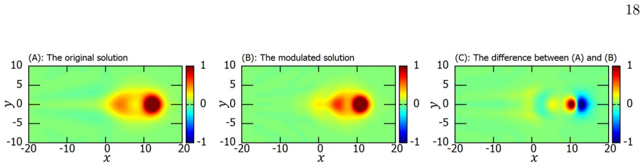
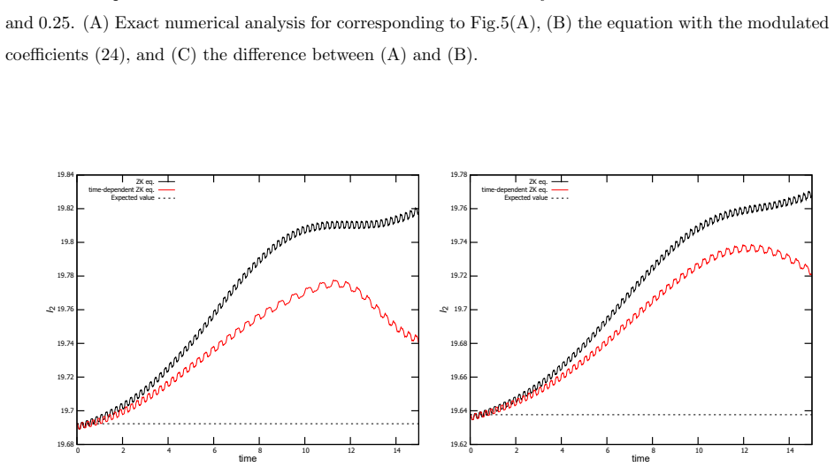
- Solving the equation with the fitted time-dependent coefficients improves I2 conservation and makes the colliding solitons keep their shape better after impact, pointing toward a variable-coefficient equation for the DIFC.
- Iterating this fit-and-resolve cycle moves the coefficients further, suggesting a self-consistent fixed-point equation that could be the true equation of the collision process.
Reading between the lines
- The authors leave implicit that the same segment-wise inverse procedure could be run on an integrable equation (e.g., KdV or NLS) as a control; if the fitted coefficients stayed constant there, it would sharpen the claim that this modulation is peculiar to quasi-integrable systems.
- A testable extension of the DIFC idea is to ask whether the fitted time-dependent coefficients are absorbing omitted effects such as radiation emission; comparing the fitted equation's output against a direct numerical simulation with resolved radiation would say whether the interaction is genuinely emergent or simply an effective model.
- The iterative refitting loop is essentially a fixed-point iteration for the effective equation; a practical improvement would be to let the coefficients be continuous functions trained jointly with the network, which could lower the reported roughly 75-hour cost per iteration step.
Editorial analysis
A structured set of objections, weighed in public.
Referee Report
Summary. The paper applies Physics-Informed Neural Networks (PINNs) and conservative PINNs (cPINNs) to forward and inverse problems for the 2+1 Zakharov-Kuznetsov (ZK) equation. For single-soliton data, the forward PINN/cPINN solutions match Runge-Kutta solutions, and inverse PINNs recover the equation coefficients (lambda_0, lambda_1) close to (2,1). For two-soliton collisions, the authors observe that the conserved quantity I2 computed by the Runge-Kutta method does not converge as the x-grid is refined and conclude that the collision configuration is not a solution of the constant-coefficient ZK equation, introducing the term 'dynamically incompatible field configuration' (DIFC). They then perform segment-wise inverse PINN analyses to infer time-dependent coefficients, interpret the coefficient modulation as an emergent effective interaction, and show that a time-dependent ZK equation improves I2 conservation.
Significance. The paper makes a methodological contribution through its multi-time-segment cPINN formulation with an adaptive conservation-loss weight, and the 1-soliton inverse results in Table I are clean and internally consistent. However, the central conceptual claim is not supported by the evidence presented. Since I2 is an exact invariant of the ZK equation for smooth doubly periodic data, the observed I2 drift in the Runge-Kutta solutions is a numerical artifact unless convergence is demonstrated. The cPINN conservation and the time-dependent-coefficient improvements are partly enforced by construction or are in-sample validations, so they do not provide independent evidence for DIFCs or emergent interactions. The paper would need to be substantially reframed as a numerical study of conservation properties of PINN discretizations rather than a discovery of new physics.
major comments (4)
- [Sec. III A, Fig. 2] The conclusion that the two-soliton configuration is a DIFC rests on the observation that I2 computed with the Runge-Kutta method does not converge as Nx increases from 150 to 350 with Ny fixed at 200. However, I2 defined in Eq. (6) is an exact invariant of Eq. (1) for smooth doubly periodic data: dI2/dt = ∫∫ u[-2u u_x - (∇²u)_x] dxdy = 0 by integration by parts. Hence any numerical trajectory with non-constant I2 is not an accurate solution of the PDE, and the drift seen in Fig. 2 is a discretization artifact unless convergence to the PDE solution is demonstrated. The paper provides no Richardson extrapolation, no time-step refinement, and no error estimates, so the statement that 'one cannot resolve the significant discrepancy' is unsupported. A grid-convergence study in both Nx and Ny, with time-step refinement, or an integrator that conserves I2 to machine precision is required before one can conclude that the PDE itself lacks a solution for this initial data.
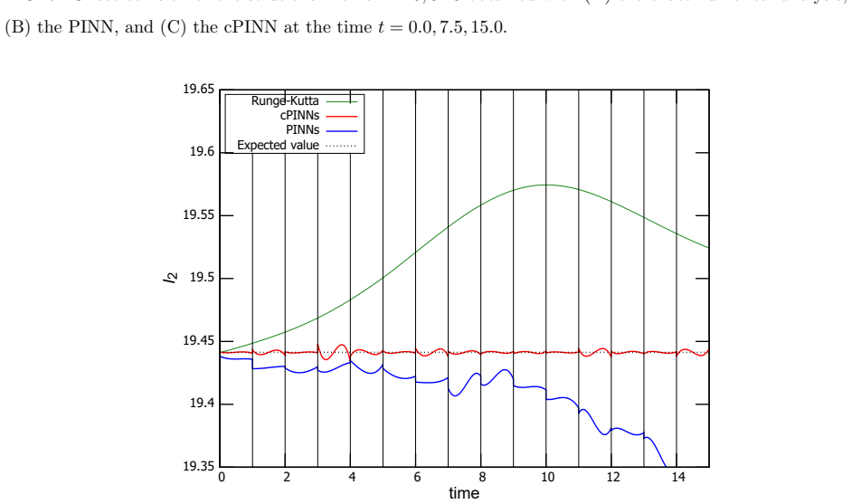
- [Sec. III A, Eq. (15), Figs. 6 and 8] The cPINN loss includes MSEC in Eq. (15), which directly penalizes deviations of the conserved quantities Ii from reference values. The near-constancy of I2 in the cPINN solutions shown in Figs. 6 and 8 is therefore enforced by construction, and the text's statement that cPINN 'identifies the solution that satisfies the conservation law' is circular unless the cPINN field is also shown to satisfy the original PDE. Fig. 11 shows that MSE_B for the cPINN is roughly an order of magnitude worse than for the PINN, so the cPINN solution is not a good solution of Eq. (1). The authors should report the relative weights of MSE_B and MSEC and evaluate the PDE residual of the cPINN output directly.
- [Sec. III E, Eqs. (24)-(25), Fig. 15] The modulated coefficients λi(t) in Eqs. (24)-(25) are fitted to cPINN training data, and the same data are then used to evaluate I2 for the time-dependent ZK equation in Fig. 15. This is an in-sample comparison; the abstract's claim that 'adherence to the laws of conservation has unquestionably improved' is not supported because a sufficiently flexible fit will always reduce the mismatch on the training set. An out-of-sample test, a hold-out time interval, or a null-model comparison (e.g., constant coefficients with the same number of fitted parameters) is needed to establish that the time dependence is meaningful.
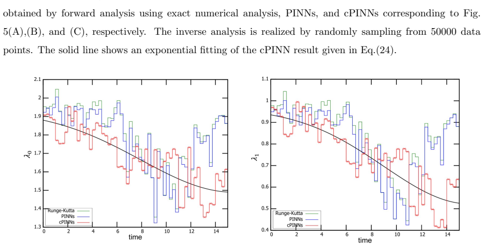
- [Sec. III C-D] The inverse analysis assumes the two-parameter form (22) and fits λ0 and λ1 segment by segment. Because the training data were generated from the constant-coefficient ZK equation, the deviations of the fitted coefficients from (2,1) can equally be explained by approximation error, optimization non-convergence, or numerical noise in the training data; no uncertainty quantification or control experiment (e.g., the same segment-wise inverse PINN applied to KdV or NLS soliton collisions) is provided. Similarly, the statement in Sec. III D that the PINN MSE of order 10^-4 indicates 'no exact solution' is a non sequitur: failure of a neural-network optimizer to reach low loss does not imply nonexistence of a PDE solution. The interpretation of the coefficient modulation as an emergent effective interaction is therefore not established.
minor comments (4)
- [Sec. I] There is a typo in the Introduction: 'Bergers eq.' should be 'Burgers equation'.
- [Fig. 14 caption] The caption of Fig. 14 says 'corresponding to Fig.5(A)', but the referenced offset collision is shown in Fig.7(A); please correct.
- [Eq. (15)] The notation I_i^{(pred),(a)} and I_i^{(correct),(a)} in Eq. (15) is not defined; please specify that a indexes time slices and describe how the Simpson integration over Np points is performed.
- [Sec. III A] The statement that I1, I3, and I4 also exhibit similar behavior to I2 is not supported by any figure or table; please provide the corresponding plots or cite specific data.
Circularity Check
The collision paper fits its time-dependent coefficients and enforces I2 conservation on the same data it then uses as confirmation, so the central 'emergent interaction' and 'improved conservation' claims are partly forced by construction; the DIFC claim additionally rests on an under-refined Runge-Kutta artifact.
-
self definitional
[Sec. II, Eq. (15); Sec. III A, Fig. 6 discussion]
"Taking into account the conservation laws Ii (i = 1, ..., 4) (5)-(8), which position the framework as a cPINN, we add to MSE (11) the following conservational contribution: MSEC := C(E) 1/Np sum |I_pred,(a)_i - I_correct,(a)_i|^2 (15) ... Fig.6 shows the conserved quantity I2 plotted over a long time scale. This demonstrates that cPINN is efficient in identifying the solution that satisfies the conservation law."
The cPINN is defined by adding MSEC, Eq. (15), which directly penalizes any deviation of the solution's I2 from the reference I2 values. Therefore the cPINN output is constructed, by definition, to conserve I2. Reporting Fig. 6 as evidence that cPINNs conserve I2 is a check that the imposed loss term was satisfied, not an independent derivation that a conservative collision solution exists. The success metric (I2 conservation) is identical to the training constraint, so the demonstration is circular.
-
fitted input called prediction
[Sec. III E, Eqs. (23)-(25) and Fig. 15; Abstract]
"we here employ a simple exponential fitting of the coefficients as lambda_i = a_i - exp(b_i + c_i t + d_i t^2), i = 0, 1 (23) with the eight fitting parameters a_i, b_i, c_i, d_i. We choose cPINN training data in this analysis ... Using the obtained DIFC, we evaluate the conservation quantity I2 and plot the time dependence in Fig.15. There is still a large discrepancy, but the quantity tends to revert to the expected exact value, unlike the result using the original equation (Fig.2)."
The time-dependent coefficients lambda_i(t) are fitted to the inverse-PINN outputs obtained from the very same collision data (cPINN data) used to define the 'DIFC'. Solving the modified equation with these fitted coefficients and then measuring improved I2 is an in-sample validation: the eight free parameters per coefficient are chosen to absorb exactly the residual of that data. The abstract's claim that 'the adherence to the laws of conservation has unquestionably improved' is therefore a goodness-of-fit statement, not an out-of-sample prediction. The improvement is statistically forced by the fitting procedure rather than independently confirmed.
full rationale
The paper has an independent and clean result: the 1-soliton inverse recovery in Table I returns lambda_0 ~ 2 and lambda_1 ~ 1 from exact, PINN, and cPINN data, demonstrating that the inverse machinery works in a controlled setting. The collision claims, however, are partly circular. The cPINN is defined by adding MSEC (Eq. 15), which directly enforces I2, so the cPINN's I2 conservation in Fig. 6 is imposed by construction. The modulated coefficients (Eqs. 23-25) are exponential fits to inverse-PINN output from the same collision data, and the improved I2 shown in Fig. 15 is then presented as confirmation; this is in-sample fitting, not prediction. The additional DIFC inference from Fig. 2 is a correctness risk because I2 is an exact invariant of Eq. (1) and no grid-convergence or error estimate is supplied, but that is not itself a circular step. There is no load-bearing self-citation chain: Refs. [31] and [48] are contextual prior work. Overall score 6 reflects partial circularity in the collision-validation loop, while the 1-soliton parameter recovery and forward PINN solutions retain independent content.
Assumptions & free parameters
free parameters (6)
- gamma =
3000
- Ecrit =
5.0e-3
- lambda_0 (nonlinear coefficient) =
varies in time, asymptotic values around 1.89-1.93 in fits (24)-(26)
- lambda_1 (dispersive coefficient) =
varies in time, asymptotic values around 0.89-0.97 in fits (24)-(26)
- exponential fit parameters a_i, b_i, c_i, d_i =
values in Eqs. (24)-(26)
- Np =
11
assumptions (4)
- domain assumption The RK4 solution with Nx up to 350 approximates the true PDE solution in the continuum limit
- standard math The ZK equation has exactly four conserved quantities I1-I4 (Eqs. 5-8)
- ad hoc to paper The time-dependence of coefficients can be represented by the exponential form (23)
- domain assumption Enforcing I2 in the loss function yields a valid solution of a physical equation
invented entities (2)
-
Dynamically incompatible field configuration (DIFC)
-
Emergent effective interaction
Cite this review
Pith. "Pith review of Inelastic Scattering, Emergent Interactions of Solitons in the Zakharov-Kuznetsov Equation through Conservative and non-Conservative Physics-Informed Neural Networks." pith.science (2026). https://pith.science/paper/C7Z3KEOY
@misc{pith2026241220027,
  author       = {Pith},
  title        = {Pith review of: Inelastic Scattering, Emergent Interactions of Solitons in the Zakharov-Kuznetsov Equation through Conservative and non-Conservative Physics-Informed Neural Networks},
  year         = {2026},
  howpublished = {\url{https://pith.science/paper/C7Z3KEOY}},
  note         = {Machine review of arXiv:2412.20027}
}
read the original abstract
The Zakharov-Kuznetsov equation, originally a three dimensional mathematical model of plasma with a uniform magnetic field, is a direct extension of the KdV equation into higher dimensions and is a typical quasi-integrable system. Physics-Informed Neural Networks (PINNs) are used to study the collision of soliton solutions in the 2+1 dimensional Zakharov-Kuznetsov equation. PINNs are able to successfully solve the equations in the forward process, and the solutions are obtained using a mesh-free approach and automatic differentiation, taking into account conservation laws. In the inverse process, the proper form of the equation can be successfully derived from a given training data. However, the situation becomes intractable in the collision process. The forward analysis result no longer adheres to the laws of conservation, and is better described as a dynamically incompatible field configuration (DIFC) than a solution to the system. Conservative PINNs have thus been introduced for this purpose, and in this paper we succeed in obtaining solutions that satisfy conservation laws. The inverse analysis suggests a different equation in which the coefficients exhibit significant changes, implying an emergence of temporary interactions. With these modulated coefficients, we recalculate the equation and confirm that the adherence to the laws of conservation has unquestionably improved.
Figures


Figures from the paper (14 more)








Forward citations
Cited by 1 Pith paper
-
PINNs Study for the Bekki-Nozaki Chaos in the Non-linear Schr\"{o}dinger equation
PINNs reproduce the Bekki-Nozaki chaotic attractor and recover NLS coefficients while the solution keeps bouncing; after decay, short-segment identification degrades.
Reference graph
Works this paper leans on
-
[1]
Hidden fluid mechanics: Learn- ing velocity and pressure fields from flow visualizations,
Maziar Raissi, Alireza Yazdani, and George Em Karniadakis, “Hidden fluid mechanics: Learn- ing velocity and pressure fields from flow visualizations,” Science 367, 1026–1030 (2020), https://www.science.org/doi/pdf/10.1126/science.aaw4741
-
[2]
Machine learning for fluid mechanics,
Steven L. Brunton, Bernd R. Noack, and Petros Koumoutsakos, “Machine learning for fluid mechanics,” Annual Review of Fluid Mechanics 52, 477–508 (2020)
work page 2020
-
[3]
Physics-informed neural networks for solving nonlinear diffusivity and biot’s equations,
Teeratorn Kadeethum, Thomas M. Jorgensen, and Hamidreza M. Nick, “Physics-informed neural networks for solving nonlinear diffusivity and biot’s equations,” PLOS ONE 15, 1–28 (2020)
work page 2020
-
[4]
Physics-informed neural networks (pinns) for fluid mechanics: a review,
Mao Zhiping Wang Zhicheng Yin Minglang Karniadakis George Em Cai, Shengze, “Physics-informed neural networks (pinns) for fluid mechanics: a review,” Acta Mechanica Sinica (2021), 10.1007/s10409- 021-01148-1
doi:10.1007/s10409- 2021
-
[5]
Physics-informed machine learning: case studies for weather and climate model- ing,
Kashinath K et al., “Physics-informed machine learning: case studies for weather and climate model- ing,” Phil.Trans.R.Soc.A 379, 20200093 (2021)
work page 2021
-
[6]
Cai S. Li H. Karniadakis G.E Jin, X., “NSFnets (NavierStokes flow nets): Physics-informed neural net- works for the incompressible Navier-Stokes equations,” Journal of Computational Physics 426, 109951 (2021)
work page 2021
-
[7]
Jiale Linghu, Weifeng Gao, Hao Dong, and Yufeng Nie, “Higher-order multi-scale physics-informed neural network (homs-pinn) method and its convergence analysis for solving elastic problems of au- thentic composite materials,” Journal of Computational and Applied Mathematics 456, 116223 (2025)
work page 2025
-
[8]
Ali Alhubail, Marwan Fahs, Fran¸ cois Lehmann, and Hussein Hoteit, “Modeling fluid flow in heteroge- neous porous media with physics-informed neural networks: Weighting strategies for the mixed pressure head-velocity formulation,” Advances in Water Resources 193, 104797 (2024)
work page 2024
Show all 75 references
-
[9]
The modified physics-informed neural network (pinn) method for the thermoelastic wave propagation analysis based on the moore-gibson-thompson theory in porous materials,
Katayoun Eshkofti and Seyed Mahmoud Hosseini, “The modified physics-informed neural network (pinn) method for the thermoelastic wave propagation analysis based on the moore-gibson-thompson theory in porous materials,” Composite Structures 348, 118485 (2024)
2024
-
[10]
A physics-informed neural network framework for multi-physics coupling microfluidic problems,
Runze Sun, Hyogu Jeong, Jiachen Zhao, Yixing Gou, Emilie Sauret, Zirui Li, and Yuantong Gu, “A physics-informed neural network framework for multi-physics coupling microfluidic problems,” Com- puters and Fluids 284, 106421 (2024)
2024
-
[11]
Driven by data or derived through physics? a review of hybrid 24 physics guided machine learning techniques with cyber-physical system (cps) focus,
Rahul Rai and Chandan K. Sahu, “Driven by data or derived through physics? a review of hybrid 24 physics guided machine learning techniques with cyber-physical system (cps) focus,” IEEE Access 8, 71050–71073 (2020)
2020
-
[12]
Variational Koop- man models: Slow collective variables and molecular kinetics from short off-equilibrium simula- tions,
Hao Wu, Feliks N¨ uske, Fabian Paul, Stefan Klus, P´ eter Koltai, and Frank No´ e, “Variational Koop- man models: Slow collective variables and molecular kinetics from short off-equilibrium simula- tions,” The Journal of Chemical Physics 146, 154104 (2017), https://pubs.aip.or...
2017 doi
-
[13]
Machine learning in cardiovascular flows modeling: Predicting arterial blood pressure from non- invasive 4d flow mri data using physics-informed neural networks,
Georgios Kissas, Yibo Yang, Eileen Hwuang, Walter R. Witschey, John A. Detre, and Paris Perdikaris, “Machine learning in cardiovascular flows modeling: Predicting arterial blood pressure from non- invasive 4d flow mri data using physics-informed neural networks,” Computer Meth...
2020
-
[14]
Physics-informed neural networks to learn cardiac fiber orientation from multiple electroanatomical maps,
Carlos Ruiz Herrera, Thomas Grandits, Gernot Plank, Paris Perdikaris, and Simone Sahli Costa- bal, Francisco andPezzuto, “Physics-informed neural networks to learn cardiac fiber orientation from multiple electroanatomical maps,” Engineering with Computers 38, 3957–3973 (2022)
2022
-
[15]
Physics-informed neural networks for modeling physiological time series for cuffless blood pressure estimation,
Mohammadi Amirmohammad Pettigrew Roderic I. Jafari Roozbeh Sel, Kaan, “Physics-informed neural networks for modeling physiological time series for cuffless blood pressure estimation,” npj Digital Medicine 6, 110 (2023)
2023
-
[16]
Physics informed deep learning (part i): Data-driven solutions of nonlinear partial differential equations,
Maziar Raissi, Paris Perdikaris, and George Karniadakis, “Physics informed deep learning (part i): Data-driven solutions of nonlinear partial differential equations,” (2017), 10.48550/arXiv.1711.10561
-
[17]
Physics informed deep learning (part ii): Data-driven discovery of nonlinear partial differential equations,
Maziar Raissi, Paris Perdikaris, and George Karniadakis, “Physics informed deep learning (part ii): Data-driven discovery of nonlinear partial differential equations,” (2017), 10.48550/arXiv.1711.10566
-
[18]
Physics-informed neural networks: A deep learning framework for solving forward and inverse problems involving nonlinear partial differential equations,
M. Raissi, P. Perdikaris, and G.E. Karniadakis, “Physics-informed neural networks: A deep learning framework for solving forward and inverse problems involving nonlinear partial differential equations,” Journal of Computational Physics 378, 686–707 (2019)
2019
-
[19]
A physics-informed neural network framework for pdes on 3d surfaces: Time independent problems,
Zhiwei Fang and Justin Zhan, “A physics-informed neural network framework for pdes on 3d surfaces: Time independent problems,” IEEE Access 8, 26328–26335 (2020)
2020
-
[20]
Delta-pinns: Physics-informed neu- ral networks on complex geometries,
Francisco Sahli Costabal, Simone Pezzuto, and Paris Perdikaris, “Delta-pinns: Physics-informed neu- ral networks on complex geometries,” Engineering Applications of Artificial Intelligence 127, 107324 (2024)
2024
-
[21]
Deep fuzzy physics- informed neural networks for forward and inverse pde problems,
Wenyuan Wu, Siyuan Duan, Yuan Sun, Yang Yu, Dong Liu, and Dezhong Peng, “Deep fuzzy physics- informed neural networks for forward and inverse pde problems,” Neural Networks 181, 106750 (2025)
2025
-
[22]
Conservative physics-informed neu- ral networks on discrete domains for conservation laws: Applications to forward and inverse problems,
Ameya D. Jagtap, Ehsan Kharazmi, and George Em Karniadakis, “Conservative physics-informed neu- ral networks on discrete domains for conservation laws: Applications to forward and inverse problems,” Computer Methods in Applied Mechanics and Engineering 365, 113028 (2020)
2020
-
[23]
Physics informed neural networks for simulating radiative transfer,
Siddhartha Mishra and Roberto Molinaro, “Physics informed neural networks for simulating radiative transfer,” Journal of Quantitative Spectroscopy and Radiative Transfer 270, 107705 (2021)
2021
-
[24]
Using physics informed neural networks for supernova radiative transfer simulation,
Xingzhuo Chen, David J. Jeffery, Ming Zhong, Levi D. McClenny, Ulisses M. Braga-Neto, and Lifan Wang, “Using physics informed neural networks for supernova radiative transfer simulation,” (2022). 25
2022
-
[25]
A data-enabled physics-informed neural network with comprehensive numerical study on solving neutron diffusion eigenvalue problems,
Yu Yang, Helin Gong, Shiquan Zhang, Qihong Yang, Zhang Chen, Qiaolin He, and Qing Li, “A data-enabled physics-informed neural network with comprehensive numerical study on solving neutron diffusion eigenvalue problems,” Annals of Nuclear Energy 183, 109656 (2023)
2023
-
[26]
Hybrid quantum physics-informed neural networks for simulating computational fluid dy- namics in complex shapes,
Alexandr Sedykh, Maninadh Podapaka, Asel Sagingalieva, Karan Pinto, Markus Pflitsch, and Alexey Melnikov, “Hybrid quantum physics-informed neural networks for simulating computational fluid dy- namics in complex shapes,” Machine Learning: Science and Technology 5, 025045 (2024)
2024
-
[27]
A two-stage physics-informed neural network method based on conserved quantities and applications in localized wave solutions,
Shuning Lin and Yong Chen, “A two-stage physics-informed neural network method based on conserved quantities and applications in localized wave solutions,” Journal of Computational Physics 457, 111053 (2022)
2022
-
[28]
Data-driven soliton solutions and model parameters of nonlinear wave models via the conservation-law constrained neural network method,
Yin Fang, Gang-Zhou Wu, Nikolay A. Kudryashov, Yue-Yue Wang, and Chao-Qing Dai, “Data-driven soliton solutions and model parameters of nonlinear wave models via the conservation-law constrained neural network method,” Chaos, Solitons and Fractals 158, 112118 (2022)
2022
-
[29]
Prediction of optical solitons using an improved physics-informed neural network method with the conservation law constraint,
Gang-Zhou Wu, Yin Fang, Nikolay A. Kudryashov, Yue-Yue Wang, and Chao-Qing Dai, “Prediction of optical solitons using an improved physics-informed neural network method with the conservation law constraint,” Chaos, Solitons and Fractals 159, 112143 (2022)
2022
-
[30]
Exactly conservative physics-informed neural networks and deep operator networks for dynamical systems,
Elsa Cardoso-Bihlo and Alex Bihlo, “Exactly conservative physics-informed neural networks and deep operator networks for dynamical systems,” Neural Networks 181, 106826 (2025)
2025
-
[31]
Discovery of Quasi-Integrable Equations from traveling-wave data using the Physics-Informed Neural Networks,
A. Nakamula, N. Obuse, N. Sawado, K. Shimasaki, Y. Shimazaki, Y. Suzuki, and K. Toda, “Discovery of Quasi-Integrable Equations from traveling-wave data using the Physics-Informed Neural Networks,” (2024), arXiv:2410.19014 [physics.flu-dyn]
2024 arXiv
-
[32]
A deep learning method for solving third-order nonlinear evolution equations,
Jun Li and Yong Chen, “A deep learning method for solving third-order nonlinear evolution equations,” Communications in Theoretical Physics 72, 115003 (2020)
2020
-
[33]
Lax pairs informed neural networks solving integrable systems,
J.C.Pu and Y.Chen, “Lax pairs informed neural networks solving integrable systems,” J. Comput. Phys. 510, 113090 (2024)
2024
-
[34]
Parallel Physics-Informed Neural Networks Method with Regularization Strategies for the Forward-Inverse Problems of the Variable Coefficient Modified KdV Equation,
Zhou Huijuan, “Parallel Physics-Informed Neural Networks Method with Regularization Strategies for the Forward-Inverse Problems of the Variable Coefficient Modified KdV Equation,” J. Syst. Sci. Complex. 37, 511–544 (2024)
2024
-
[35]
Physics-informed neural network methods based on miura transforma- tions and discovery of new localized wave solutions,
Shuning Lin and Yong Chen, “Physics-informed neural network methods based on miura transforma- tions and discovery of new localized wave solutions,” Physica D: Nonlinear Phenomena 445, 133629 (2023)
2023
-
[36]
Solving forward and inverse problems of the logarithmic nonlinear schr¨ odinger equation with pt-symmetric harmonic potential via deep learning,
Zijian Zhou and Zhenya Yan, “Solving forward and inverse problems of the logarithmic nonlinear schr¨ odinger equation with pt-symmetric harmonic potential via deep learning,” Physics Letters A387, 127010 (2021)
2021
-
[37]
Solving localized wave solutions of the derivative nonlinear schr¨ odinger equation using an improved pinn method,
Juncai Pu, Jun Li, and Yong and Chen, “Solving localized wave solutions of the derivative nonlinear schr¨ odinger equation using an improved pinn method,” Nonlinear Dynamics105, 1723–1739 (2021)
2021
-
[38]
Advanced physics-informed neural networks for numerical approximation of the coupled schr¨ odinger–kdv equation,
Qiongni Zhang, Changxin Qiu, Jiangyong Hou, and Wenjing Yan, “Advanced physics-informed neural networks for numerical approximation of the coupled schr¨ odinger–kdv equation,” Communications in 26 Nonlinear Science and Numerical Simulation 138, 108229 (2024)
2024
-
[39]
Physics-informed neural networks method in high-dimensional integrable sys- tems,
Z.W.Miao and Y.Chen, “Physics-informed neural networks method in high-dimensional integrable sys- tems,” Mod.Phys.Lett.B. 36(1), 2150531 (2022)
2022
-
[40]
Deep neural networks learning forward and inverse problems of two-dimensional nonlinear wave equations with rational solitons,
Zijian Zhou, Li Wang, and Zhenya Yan, “Deep neural networks learning forward and inverse problems of two-dimensional nonlinear wave equations with rational solitons,” Computers and Mathematics with Applications 151, 164–171 (2023)
2023
-
[41]
Data-driven vortex solitons and parameter discovery of 2d generalized nonlinear schr¨ odinger equations with a pt-symmetric optical lattice,
Li Wang, Zijian Zhou, and Zhenya Yan, “Data-driven vortex solitons and parameter discovery of 2d generalized nonlinear schr¨ odinger equations with a pt-symmetric optical lattice,” Computers and Mathematics with Applications 140, 17–23 (2023)
2023
-
[42]
Physics informed neural net- works (pinns) for approximating nonlinear dispersive pdes,
UjjwalMishra Siddhartha Bai, GenmingKoley and Roberto Molinaro, “Physics informed neural net- works (pinns) for approximating nonlinear dispersive pdes,” Journal of Computational Mathematics 39, 816–847 (2021)
2021
-
[43]
Deep neural networks learning forward and inverse problems of two- dimensional nonlinear wave equations with rational solitons,
Z.Y. Yan Z.J. Zhou, L. Wang, “Deep neural networks learning forward and inverse problems of two- dimensional nonlinear wave equations with rational solitons,” Comput. Math. Appl. 151, 164–171 (2023)
2023
-
[44]
Three-dimensional solitons,
V. Zakharov and E A. Kuznetsov, “Three-dimensional solitons,” Soviet Physics JETP 29, 594–597 (1974)
1974
-
[45]
Cylindrical quasi-solitons of the Zakharov- Kuznetsov equation,
Hiroshi Iwasaki, Sadayoshi Toh, and Takuji Kawahara, “Cylindrical quasi-solitons of the Zakharov- Kuznetsov equation,” Physica D: Nonlinear Phenomena 43, 293–303 (1990)
1990
-
[46]
Bilayer vortices in rotating stratified fluid,
V. I. Petviashvili and V. V. Yan’kov, “Bilayer vortices in rotating stratified fluid,” Dokl. Akad. Nauk SSSR 267, 825–828 (1982)
1982
-
[47]
Numerical study of Zakhavor-Kuznetsov equations in two dimensions,
Christian Klein, Svetlana Roudenko, and Nikola Stoilov, “Numerical study of Zakhavor-Kuznetsov equations in two dimensions,” Journal of Nonlinear Science 31, 1–28 (2021)
2021
-
[48]
Mock-integrability and stable solitary vortices,
Yukito Koike, Atsushi Nakamula, Akihiro Nishie, Kiori Obuse, Nobuyuki Sawado, Yamato Suda, and Kouichi Toda, “Mock-integrability and stable solitary vortices,” Chaos Solitons and Fractals: the in- terdisciplinary journal of Nonlinear Science and Nonequilibrium and Complex Phen...
2022 arXiv
-
[49]
One more example of inelastic soliton interaction,
Kh.O. Abdulloev, I.L. Bogolubsky, and V.G. Makhankov, “One more example of inelastic soliton interaction,” Physics Letters A 56, 427–428 (1976)
1976
-
[50]
Resonant production of solitons in the rlw equation,
J. Courtenay Lewis and J.A. Tjon, “Resonant production of solitons in the rlw equation,” Physics Letters A 73, 275–279 (1979)
1979
-
[51]
Quasi-integrability of deformations of the KdV equation,
F. ter Braak, L. A. Ferreira, and W. J. Zakrzewski, “Quasi-integrability of deformations of the KdV equation,” Nucl. Phys. B 939, 49–94 (2019), arXiv:1710.00918 [hep-th]
2019 arXiv
-
[52]
Interactions of two-dimensionally localized pulses of the regularized-long-wave equation,
Takuji Kawahara, Keisuke Araki, and Sadayoshi Toh, “Interactions of two-dimensionally localized pulses of the regularized-long-wave equation,” Physica D: Nonlinear Phenomena 59, 79–89 (1992)
1992
-
[53]
Model equations for long waves in nonlinear dispersive systems,
Thomas Brooke Benjamin, J. L. Bona, and J. J. Mahony, “Model equations for long waves in nonlinear dispersive systems,” Philosophical Transactions of the Royal Society of London. Series A, Mathematical 27 and Physical Sciences 272, 47–78 (1972)
1972
-
[54]
Soliton stability in plasmas and hydrodynam- ics,
E.A. Kuznetsov, A.M. Rubenchik, and V.E. Zakharov, “Soliton stability in plasmas and hydrodynam- ics,” Physics Reports 142, 103–165 (1986)
1986
-
[55]
On the limited memory bfgs method for large scale optimization,
Dong C. Liu and Jorge Nocedal, “On the limited memory bfgs method for large scale optimization,” Mathematical Programming 45, 503–528 (1989)
1989
-
[56]
Physics-informed neural networks for the shallow-water equations on the sphere,
Alex Bihlo and Roman O. Popovych, “Physics-informed neural networks for the shallow-water equations on the sphere,” Journal of Computational Physics 456, 111024 (2022)
2022
-
[57]
Characterizing possible failure modes in physics-informed neural networks,
Aditi S. Krishnapriyan, Amir Gholami, Shandian Zhe, Robert M. Kirby, and Michael W. Mahoney, “Characterizing possible failure modes in physics-informed neural networks,” Proceedings of the 35th International Conference on Neural Information Processing Systems, NIPS ’21 (2024)
2024
-
[58]
Numerical studies of the regularized long wave equation,
Katuhiko Goda and Yoshinari Fukui, “Numerical studies of the regularized long wave equation,” Journal of the Physical Society of Japan 48, 623–630 (1980), https://doi.org/10.1143/JPSJ.48.623
1980 doi
-
[59]
Dynamics of two-dimensional solitary vortices in a low- beta plasma with convective motion,
Mitsuhiro Makino, Tetsuo Kamimura, and Tosiya Taniuti, “Dynamics of two-dimensional solitary vortices in a low- beta plasma with convective motion,” Journal of the Physical Society of Japan 50, 980–989 (1981), https://doi.org/10.1143/JPSJ.50.980
1981 doi
-
[60]
The concept of quasi-integrability,
L. A. Ferreira, G. Luchini, and Wojtek J. Zakrzewski, “The concept of quasi-integrability,” AIP Conf. Proc. 1562, 43–49 (2013), arXiv:1307.7722 [hep-th]
2013 arXiv
-
[61]
Extended physics-informed neural networks (xpinns): A generalized space-time domain decomposition based deep learning framework for nonlinear partial differential equations,
Ameya D. Jagtap and George Em Karniadakis, “Extended physics-informed neural networks (xpinns): A generalized space-time domain decomposition based deep learning framework for nonlinear partial differential equations,” Communications in Computational Physics 28, 2002–2041 (2020)
2020
-
[62]
Iterative algorithms for partitioned neural network approximation to partial differential equations,
Hee Jun Yang and Hyea Hyun Kim, “Iterative algorithms for partitioned neural network approximation to partial differential equations,” Computers and Mathematics with Applications 170, 237–259 (2024)
2024
-
[63]
Exact solution via the spectral transform of a generalization with linearly x-dependent coefficients of the modified korteweg-de-vries equation,
F. Calogero and Ao Degasperis, “Exact solution via the spectral transform of a generalization with linearly x-dependent coefficients of the modified korteweg-de-vries equation,” Lett. Nuovo Cim 22, 270–273 (1978)
1978
-
[64]
The integration of burgers and korteweg-de vries equations with nonuni- formities,
T. Brugarino and P. Pantano, “The integration of burgers and korteweg-de vries equations with nonuni- formities,” Physics Letters A 80, 223–224 (1980)
1980
-
[65]
Painlev´ e property of general variable-coefficient versions of the korteweg-de vries and non-linear schr¨ odinger equations,
Nalini Joshi, “Painlev´ e property of general variable-coefficient versions of the korteweg-de vries and non-linear schr¨ odinger equations,” Physics Letters A125, 456–460 (1987)
1987
-
[66]
Painlev´ e analysis of nonautonomous evolution equations,
Ladislav Hlavat` y, “Painlev´ e analysis of nonautonomous evolution equations,” Physics Letters A128, 335–338 (1988)
1988
-
[67]
Painlev´ e analysis and reducibility to the canonical form for the generalized kadomtsev–petviashvili equation,
Tommaso Brugarino and Antonio M. Greco, “Painlev´ e analysis and reducibility to the canonical form for the generalized kadomtsev–petviashvili equation,” Journal of mathematical physics 32, 69–71 (1991)
1991
-
[68]
Variable-coefficient balancing-act algorithm extended to a variable- coefficient mkp model for the rotating fluids,
Yi-Tian Gao and Bo Tian, “Variable-coefficient balancing-act algorithm extended to a variable- coefficient mkp model for the rotating fluids,” International Journal of Modern Physics C12, 1383–1389 (2001)
2001
-
[69]
A generalized kdv-family with variable coefficients in (2+ 1) 28 dimensions,
Tadashi Kobayashi and Kouichi Toda, “A generalized kdv-family with variable coefficients in (2+ 1) 28 dimensions,” IEICE Transactions on Fundamentals of Electronics, Communications and Computer Sciences 88, 2548–2553 (2005)
2005
-
[70]
The painlev´ e test and reducibility to the canonical forms for higher-dimensional soliton equations with variable-coefficients,
Tadashi Kobayashi and Kouichi Toda, “The painlev´ e test and reducibility to the canonical forms for higher-dimensional soliton equations with variable-coefficients,” SIGMA. Symmetry, Integrability and Geometry: Methods and Applications 2, 063 (2006)
2006
-
[71]
Optical waves/modes in a multicomponent inho- mogeneous optical fiber via a three-coupled variable-coefficient nonlinear schr¨ odinger system,
Xin-Yi Gao, Yong-Jiang Guo, and Wen-Rui Shan, “Optical waves/modes in a multicomponent inho- mogeneous optical fiber via a three-coupled variable-coefficient nonlinear schr¨ odinger system,” Applied Mathematics Letters 120, 107161 (2021)
2021
-
[72]
Xin-yi Gao, Yong-jiang Guo, Wen-rui Shan, Tian-yu Zhou, Meng Wang, and Dan-yu Yang, “In the atmosphere and oceanic fluids: Scaling transformations, bilinear forms, b¨ acklund transformations and solitons for a generalized variable-coefficient korteweg-de vries-modified kortewe...
2021
-
[73]
Similarity reductions for a generalized (3+1)- dimensional variable-coefficient b-type kadomtsev-petviashvili equation in fluid dynamics,
Xin-Yi Gao, Yong-Jiang Guo, and Wen-Rui Shan, “Similarity reductions for a generalized (3+1)- dimensional variable-coefficient b-type kadomtsev-petviashvili equation in fluid dynamics,” Chinese Journal of Physics 77, 2707–2712 (2022)
2022
-
[74]
In nonlinear optics, fluid mechanics, plasma physics or atmospheric science: symbolic computation on a generalized variable-coefficient korteweg-de vries equation,
Xin-Yi Gao, Yong Guo, and Wen-Rui Shan, “In nonlinear optics, fluid mechanics, plasma physics or atmospheric science: symbolic computation on a generalized variable-coefficient korteweg-de vries equation,” Acta Mathematica Sinica, English Series (2022)
2022
-
[75]
Water-wave studies on a (2+ 1)-dimensional generalized variable- coefficient boiti–leon–pempinelli system,
Xiao-Tian Gao and Bo Tian, “Water-wave studies on a (2+ 1)-dimensional generalized variable- coefficient boiti–leon–pempinelli system,” Applied Mathematics Letters 128, 107858 (2022)
2022
Reviewed August 10, 2026 · model on record in the stance chip above.
Discussion (0). Continue with ORCID to comment.