REVIEW 4 major objections 5 minor 1 cited by
Are Two Hidden Layers Still Enough for the Physics-Informed Neural Networks?
T0 review · 4 major / 5 minor · reviewed 2026-08-11 · deepseek-v4-flash
Pith's one-line read The paper argues that one-hidden-layer physics-informed networks, started from a deterministic Euler-like initialization and trained with special loss weighting, match or beat deeper baselines on a range of ODE and PDE benchmarks.
desk verdict A bag of useful tricks for shallow PINNs, but the headline SOTA claim doesn't survive the paper's own Table 7. read the letter →
The pith
A machine-rendered reading of the paper's core claim, the machinery that carries it, and where it could break.
The reading
What carries the argument
The load-bearing object is the strictly deterministic initialization (Algorithm 2). It fixes the hidden-layer weights to $W_k^{(1)}=2\Delta\zeta/\Delta x$ and biases to $b_k^{(1)}=-2(k+1)\Delta\zeta$, and sets the output-layer weights from the local derivative-matching identity $W_k^{(2)}=-2\Delta x\,N_l[u(0),x_{k+1}]/\Delta\zeta$, with the output bias equal to the initial value; the parameter $\Delta\zeta=\ln(2+\sqrt{3})/2$ is chosen so that the third derivative of neighboring sigmoids cancels at each neuron center. This construction makes the initial network an Euler-like piecewise-sigmoid integrator, so the subsequent training stages only refine a good starting representation. The separable extension for PDEs, $u_{\theta}(t,x)=\sum_j v_j(t)w_j(x)$, is the second central object: it lets the same one-hidden-layer construction be applied along each coordinate and combined multiplicatively, which is what the paper calls a two-hidden-layer SPINN.
What would settle it
Freeze the hidden layer after Algorithm 2 on an ODE with a known analytic solution, compute the full derivative sum in Eq. (14) at every grid point, and compare it to the one-neuron approximation in Eq. (15). If the relative mismatch is large, say above 10%, on any part of the domain—especially with $\Delta\zeta=\ln(2+\sqrt{3})/2$—then the localization assumption that underlies the output-weight formula is broken, and the claimed source of the method's accuracy is not present.
Extended reading notes
Core claim
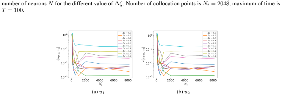
The paper's central claim is that the expressive power of deep PINNs is not needed for the problems considered: a single-hidden-layer network, whose hidden weights and biases are fixed rather than learned and whose output weights are set from the ODE residual at grid points, can be trained to competitive accuracy, and its product with a second single-hidden-layer network (the separable SPINN architecture) extends the same construction to two-dimensional PDEs. The deterministic initialization is derived from the Euler method: with $W_k^{(1)}=2\Delta\zeta/\Delta x$ and $b_k^{(1)}=-2(k+1)\Delta\zeta$, the $k$th sigmoid's steepest response sits at $x_{k+1}$, and assuming that one neuron dominates the derivative at each grid point gives $W_k^{(2)}=-2\Delta x\,N_l[u(0),x_{k+1}]/\Delta\zeta$. The paper chooses $\Delta\zeta=\ln(2+\sqrt{3})/2\approx 0.66$ so that third-derivative interference between neighboring sigmoids cancels, and confirms experimentally that $\Delta\zeta\approx 0.7$ works best. On top of this initialization the paper adds loss-weighting schemes—detaching nonlinear operators, second-derivative weighting, predicted-solution-based weighting, relative residuals, δ-causal training, and gradient normalization—plus a data-driven variant called PIDD initialization and a gradient-free neuron-by-neuron fitting rule. The empirical payoff is reported as competitive accuracy across ODE and PDE benchmarks and, for the Lorenz system, errors below the causal-training baseline quoted in the paper.
Load-bearing premise
The load-bearing premise is that each sigmoid neuron responds mainly at its own grid point, so the network derivative at a point is essentially one neuron's contribution; if neighboring sigmoids overlap heavily, the deterministic start is not a faithful Euler-like approximation and training must repair a bad representation.
Editorial extensions
If this is right
- For ODEs, the deterministic initialization alone improves the harmonic-oscillator relative L2 error by an order of magnitude over random output-layer initialization, from about 4.7e-3 to 7.7e-4, and the full training pipeline brings it to roughly 2.2e-4.
- The combination of detaching, δ-causal weighting, second-derivative weighting, and gradient normalization turns the relativistic-slingshot problem from unusable errors into errors around 1e-3 to 1e-2, with relative L2 values such as 1.2e-3 for h and 1.3e-3 for x.
- Predicted-solution-based weighting or relative-residual weighting extends accurate solutions to multi-scale regimes where plain training fails, e.g., exponential growth on [0,10] improves from 0.93 to 1.72e-3, and the Lorenz system on [0,20] reaches errors around 5e-4 to 8e-4.
- The gradient-free neuron-by-neuron fitting method reaches Lorenz-system errors below the causal-training baseline reported in the paper (x: 9.8e-4, y: 1.4e-3, z: 6.0e-4) after three sweeps over neurons and without using an optimizer.
- On the Allen–Cahn PDE, the two-hidden-layer separable SPINN with deterministic initialization and the full weighting stack reaches relative L2 error 4.40e-5, below the δ-causal training baseline of 6.29e-5 listed in the paper.
Reading between the lines
- Editorial inference: the Euler-matching initialization effectively replaces random weight guessing with a discretization prior, so the trained network should inherit the convergence order and error profile of a first-order integrator; one testable consequence is that halving the grid step should roughly halve the error floor before optimization, which the paper's scaling plots hint at but do not a
- Editorial inference: because only output weights are set analytically and hidden weights stay frozen during the first training stages, the method invites an extreme-learning-machine-style analysis; the paper notes this connection itself, but a rigorous approximation-rate bound for the sigmoid Euler construction is left open.
- Editorial inference: the generalization measure introduced in the paper, which compares errors on training parameters versus half-shifted parameters, could be applied to any parameterized PINN, not just the separable construction; the low value in the chaotic Lorenz regime suggests the generalization claim should be read as confined to regular parameter regions.
- Editorial inference: the same deterministic initialization could be extended beyond the tested equations to systems with stiffness or shocks by replacing the uniform grid with adaptive collocation points; nothing in the derivation requires uniformity, so adaptive grid spacing is a natural next experiment.
Editorial analysis
A structured set of objections, weighed in public.
Referee Report
Summary. The paper proposes a set of initialization, weighting, and training techniques for physics-informed neural networks with one hidden layer, and for separable PINNs (SPINN) with two such layers, for solving ODEs and PDEs. The contributions include a 'strictly deterministic' initialization (Algorithms 1–2), modifications of causal training and gradient normalization, new loss-weighting schemes (detaching, second-derivative weighting, PSBW, RR), a physics-informed data-driven (PIDD) initialization that fits the network to precomputed reference data (Algorithm 3), a generalization metric for parameterized problems (Appendix B), a gradient-free neuron-by-neuron (NbN) fitting algorithm (Algorithm 5), and an extension to 2D problems using SPINN. The central claim, stated in the abstract and conclusions, is that these shallow networks achieve competitive accuracy and, in some cases, state-of-the-art results.
Significance. If the claims are substantiated, the paper would make a useful contribution by demonstrating that very shallow PINNs with carefully chosen initialization and training can be a cheaper alternative to deep architectures. The paper's strengths include a large experimental campaign, concrete algorithms that are easy to reimplement, and a deterministic initialization that removes random-seed variability. The NbN method is genuinely gradient-free and the generalization metric is a step toward quantifying interpolation behavior. However, the significance is diminished by the unsupported state-of-the-art claim, the circular evaluation of PIDD, and the lack of error analysis for the heuristic approximations at the core of the initialization; these issues prevent the current manuscript from supporting its strongest conclusions.
major comments (4)
- [Abstract, Section 6, Table 7] The claim that NbN training gives 'state-of-the-art results on the Lorentz system' is not supported by the evidence presented. Table 7 reports relative L2 errors for NbN training of (9.8e-4, 1.4e-3, 6.0e-4), which are 3-5 times larger than the PIDD initialization errors (2.0e-4, 6.7e-4, 1.3e-4) listed in the same table, and the only external baseline is 'Causal training [4]'. No comparison with other recent PINN methods for the Lorenz system, no seed or error-bar statistics, and no compute-matched comparison are provided. Since this is the only concrete instance of 'state-of-the-art' offered in the paper, the abstract's central claim rests on an internally contradicted and externally unbenchmarked result.
- [Section 4.1, Algorithms 3-4, Examples 15-16 and 22-23] The PIDD initialization is data-driven: the output weights are set using solutions generated by odeint or Chebfun (e.g., Section 4.2.1 states the data were 'generated with odeint'), and the reported relative L2 errors are then computed against the same reference solutions. This makes the PIDD results an interpolation test on the training data rather than an independent solver-free PINN result. The paper should explicitly acknowledge this circularity and distinguish it from the solver-free NbN results. In particular, Table 7 should not be read as a fair comparison between PIDD and NbN, since PIDD has access to the reference data.
- [Section 2, Eqs. (14)-(16); Section 4.1, Eqs. (47)-(49)] The deterministic initialization rests on two heuristic assumptions: that the derivative of the network at x_m is dominated by a single neuron's sigma'(0) term, and that neighboring output weights vary slowly. These assumptions are not quantified, no error bounds are derived, and the key hyperparameter delta-zeta is selected empirically (Section 2.1.3 reports 'the best results were achieved at delta-zeta = 0.7'). Additionally, the derivation leading to Eq. (16) is internally inconsistent: the text derives an approximation involving W_{m-1} at x_m but then states 'we have the following equation for the weights W_m' with N evaluated at x_{m+1}. A numerical check of how well Eq. (15) holds as a function of N and delta-zeta, and a sensitivity analysis, would substantially strengthen the paper.
- [Section 4.3, Appendix B, Examples 17-18] The 'generalization' properties of the proposed network are evaluated only at the midpoints q_{i+1/2} of the training grid, i.e., as interpolation within the domain [q_min, q_max]. This is not extrapolation to unseen parameter ranges, and the paper even shows in Example 18 that the method fails to generalize in chaotic regimes (mu = 0.023 for rho in [25,30]). The claim of 'pronounced generalizing properties' should be qualified as interpolation between precomputed solution snapshots, and the metric mu should be described as an interpolation-error ratio rather than a measure of genuine generalization.
minor comments (5)
- [Throughout] The spelling 'Lorentz system' appears in Examples 16 and 20, Table 7, and the Conclusions; the correct name is 'Lorenz system' (as used in the equations and in the reference to Lorenz 1963).
- [Section 3.5.1] The paragraph 'We noticed that changing the weights lambda_ic and lambda_r can lead to better accuracy...' indicates that key hyperparameters were tuned after seeing the test results. The paper would benefit from a description of a validation or cross-validation protocol that separates hyperparameter selection from final performance evaluation.
- [Section 4.2.2, Example 16] The phrase 'under which the calculations in [4] were carried out' would be clearer if the exact reference values of sigma, rho, and beta were stated with the units or conventions used; currently the reader must infer them from the equation.
- [Appendix B, Eq. (65)] The definition of the generalization measure mu is correct but the textual description 'the ratio of the relative total L2 error of prediction of set {q_{i+1/2}} to the ratio of the relative total L2 error of prediction of set {q_i}' is garbled; it should say 'the ratio of the error on the training grid to the error on the midpoints'.
- [Figure 7 caption] The caption 'Contribution to the solution u_{theta,1} of the first 1 (a), 11 (b), 21 (c)...' is missing commas and the first item should read 'first 1 neuron (a), first 11 neurons (b), first 21 neurons (c), ...'.
Circularity Check
PIDD accuracy is a fit residual, the 'generalization' measure tests interpolation, and the loss-weighting rule is a load-bearing self-citation.
-
fitted input called prediction
[Section 4.2.1 (Example 15) and Section 4.2.2 (Example 16), with Algorithm 3]
"The reference solutions are obtained by using the odeint solver of scipy.integrate library. The data {uk}N k=0 for uniform distribution points {xk}N k=0 were generated with odeint for N = 20000 in 0.004 seconds. Results of PIDD initialization for neural network with N = 20000 are following: the relative L2 errors are ϵ[uθ;1, uref 1] = 5.67×10⁻⁵ and ϵ[uθ;2, uref 2] = 6.82×10⁻⁴."
Algorithm 3 sets each output weight to W(2)_k = −(Δx/(2Δζ)) N[u_k, x_k]/κ_k, so the output-layer parameters are algebraic functions of the reference solution u_k at the same grid points x_k. The reported relative L2 error (Appendix A, Eq. (64)) is then computed against that same reference solution u. The number therefore measures interpolation or fitting residual on the training grid, not an independent prediction; a network whose output layer is computed from the reference data is forced to match those values up to the κ localization correction. Presenting this as competitive accuracy treats a fitted input as a predicted result.
-
self definitional
[Section 4.3 (Suggestion 9, Algorithm 4) and Appendix B]
"The second set of solution values is calculated for the calculated grid of the parameter q in steps of ∆q, offset by ∆q/2, i.e. at points as far away as possible from the nearest points of q where the training was carried out, but not out of the training domain."
The Q network is constructed by least squares W(2)a = I with bump activations chosen so that Q_j(q_n) ≈ 1 at the training parameters and values close to zero for other q; hence every q in [q_min, q_max], including the midpoints q_{j+1/2}, lies inside the interpolation span of the fitted bumps. The generalization measure µ = ϵ1/ϵ1/2 therefore compares fit on the training parameter grid with interpolation at midpoints of that same grid, both strictly inside the training domain. The claimed 'pronounced generalizing properties' are, by construction, properties of an interpolant rather than extrapolation to unseen parameter regions.
1 more flagged steps
-
self citation load bearing
[Section 3.2 and Section 6, citing reference [10]]
"The original problem described by a differential equation (1) accompanied with the initial condition (2) can be reformulated to the problem described by the differential equation only. The procedure of reformulation is given in the [10]. According to this method the weights λk ic and λk r are related to each other by means of the relation λk ic = βkλk r."
Reference [10] is by the same group (Es'kin, Davydov, Egorova, Malkhanov, Akhukov, Smorkalov), and the conclusion states that 'in all numerical experiments ... the relations between λr and λic loss functions were taken based on the method proposed in [10]'. This λic = βλr relation is not re-derived or independently verified in the present paper, yet it is load-bearing for every reported training result that uses the composite loss (4). The experimental accuracy numbers therefore rest on a self-citation chain, even though the relation is not the sole determinant of the accuracy values.
full rationale
The strictly deterministic initialization (Algorithms 1–2) and the neuron-by-neuron training (Algorithm 5) are largely self-contained: the output weights are set from the ODE residual at grid points and then refined by the network's own predictions, without importing a reference solution. The central architectural claim that one or two hidden layers suffice also has independent content. However, the PIDD accuracy claims (Examples 15, 16, 22, 23) import the reference solution as the input to Algorithm 3 and then evaluate against the same reference, so those error numbers are interpolation residuals rather than independent predictions. The generalization section similarly constructs Q from the training-parameter grid and then measures at midpoints of that grid, so µ quantifies interpolation, not extrapolation. The λic = βλr weighting used throughout is taken from the authors' own prior work [10] without independent verification, making it a load-bearing self-citation. Separately, the Lorenz 'state-of-the-art' statement is weakened by the paper's own Table 7, where PIDD is 3–5x more accurate than NbN, and no external SOTA baseline is supplied; that is a correctness/support problem rather than circularity. Overall, the thesis retains independent content, but two of the headline empirical claims reduce by construction, giving a partial circularity score.
Assumptions & free parameters
free parameters (8)
- delta-zeta (Algorithm 2) =
0.7
- Loss weights lambda_ic, lambda_r =
varies per example (e.g. 1/10, 10^3/10^4, 10^5/10^6)
- Causality parameter epsilon initial =
10^-8, 10^-24, doubled with threshold delta_w = 0.99
- PSBW/RR decay gamma =
0.9 (PSBW), 0.99 (RR)
- Gradient normalization moving average alpha =
0.9
- PIDD truncation window L =
10
- beta_k relation for loss weights =
varies with problem
- Training schedules (stages, epochs, learning rates) =
varies, e.g. Adam 1e-3, LBFGS, Adam 1e-5, up to 300000 epochs
assumptions (7)
- standard math Universal approximation theorem for single-hidden-layer sigmoid networks
- ad hoc to paper A sigmoid neuron's response is localized and approximately linear on [-delta-zeta, delta-zeta]
- ad hoc to paper Derivative of the network at x_m is dominated by a single neuron's sigma'(0) term
- ad hoc to paper Output weights W^(2)_k vary slowly near index m, allowing truncation to L neighbors
- domain assumption delta-causal weighting relation beta from ref [10] is valid
- domain assumption Euler method global error O(X/N) is a guide for initialization error
- domain assumption Reference solutions from odeint/Chebfun are accurate ground truth
Cite this review
Pith. "Pith review of Are Two Hidden Layers Still Enough for the Physics-Informed Neural Networks?." pith.science (2026). https://pith.science/paper/CLLVJRXS
@misc{pith2026241219235,
  author       = {Pith},
  title        = {Pith review of: Are Two Hidden Layers Still Enough for the Physics-Informed Neural Networks?},
  year         = {2026},
  howpublished = {\url{https://pith.science/paper/CLLVJRXS}},
  note         = {Machine review of arXiv:2412.19235}
}
read the original abstract
The article discusses the development of various methods and techniques for initializing and training neural networks with a single hidden layer, as well as training a separable physics-informed neural network consisting of neural networks with a single hidden layer to solve physical problems described by ordinary differential equations (ODEs) and partial differential equations (PDEs). A method for strictly deterministic initialization of a neural network with one hidden layer for solving physical problems described by an ODE is proposed. Modifications to existing methods for weighting the loss function are given, as well as new methods developed for training strictly deterministic-initialized neural networks to solve ODEs (detaching, additional weighting based on the second derivative, predicted solution-based weighting, relative residuals). An algorithm for physics-informed data-driven initialization of a neural network with one hidden layer is proposed. A neural network with pronounced generalizing properties is presented, whose generalizing abilities of which can be precisely controlled by adjusting network parameters. A metric for measuring the generalization of such neural network has been introduced. A gradient-free neuron-by-neuron fitting method has been developed for adjusting the parameters of a single-hidden-layer neural network, which does not require the use of an optimizer or solver for its implementation. The proposed methods have been extended to 2D problems using the separable physics-informed neural networks approach. Numerous experiments have been carried out to develop the above methods and approaches. Experiments on physical problems, such as solving various ODEs and PDEs, have demonstrated that these methods for initializing and training neural networks with one or two hidden layers (SPINN) achieve competitive accuracy and, in some cases, state-of-the-art results.
Figures


Figures from the paper (33 more)






Forward citations
Cited by 1 Pith paper
-
About rectified sigmoid function for enhancing the accuracy of Physics-Informed Neural Networks
Rectified sigmoid (hard sigmoid) activation is reported to cut PINN solution errors by about an order of magnitude on two ODE benchmarks, but the result may be an interpolation artifact because the paper never disclos...
Reference graph
Works this paper leans on
-
[4]
Respecting causality is all you need for training physics-informed neural networks,
S. Wang, S. Sankaran, and P. Perdikaris, “Respecting causality is all you need for training physics-informed neural networks,” 2022. [Online]. Available: http://arxiv.org/abs/2203.07404
arXiv 2022
-
[1]
Highly accurate protein structure prediction with AlphaFold,
J. Jumper, R. Evans, A. Pritzel, T. Green, M. Figurnov, O. Ronneberger, K. Tunyasuvunakool, R. Bates, A. Žídek, A. Potapenko, A. Bridgland, C. Meyer, S. A. A. Kohl, A. J. Ballard, A. Cowie, B. Romera-Paredes, S. Nikolov, R. Jain, J. Adler, T. Back, S. Petersen, D. Reiman, E. Clancy, M. Zielinski, M. Steinegger, M. Pacholska, T. Berghammer, S. Bodenstein, ...
2021
-
[2]
A foundation model for the earth system,
C. Bodnar, W. P. Bruinsma, A. Lucic, M. Stanley, A. Vaughan, J. Brandstetter, P. Garvan, M. Riechert, J. A. Weyn, H. Dong, J. K. Gupta, K. Thambiratnam, A. T. Archibald, C.-C. Wu, E. Heider, M. Welling, R. E. Turner, and P. Perdikaris, “A foundation model for the earth system,” 2024. [Online]. Available: https://arxiv.org/abs/2405.13063
arXiv 2024
-
[3]
Physics-informed neural networks: A deep learning framework for solving forward and inverse problems involving nonlinear partial differential equations,
M. Raissi, P. Perdikaris, and G. E. Karniadakis, “Physics-informed neural networks: A deep learning framework for solving forward and inverse problems involving nonlinear partial differential equations,” Journal of Computational Physics , vol. 378, pp. 686–707, 2019. [Online]. Available: https://linkinghub.elsevier.com/retrieve/pii/S0021999118307125
2019
-
[5]
H. Wang, X. Qian, Y . Sun, and S. Song, “A Modified Physics Informed Neural Networks for Solving the Partial Differential Equation with Conservation Laws,”—. [Online]. Available: https://ssrn.com/abstract=4274376
-
[6]
Learning nonlinear operators via DeepONet based on the universal approximation theorem of operators,
L. Lu, P. Jin, G. Pang, Z. Zhang, and G. E. Karniadakis, “Learning nonlinear operators via DeepONet based on the universal approximation theorem of operators,” Nature Machine Intelligence, vol. 3, no. 3, pp. 218–229, mar
-
[7]
A General Neural- Networks-Based Method for Identification of Partial Differential Equations, Implemented on a Novel AI Accelerator,
M. A. Krinitskiy, V . M. Stepanenko, A. O. Malkhanov, and M. E. Smorkalov, “A General Neural- Networks-Based Method for Identification of Partial Differential Equations, Implemented on a Novel AI Accelerator,” Supercomputing Frontiers and Innovations , vol. 9, no. 3, sep 2022. [Online]. Available: https://superfri.org/index.php/superfri/article/view/439
2022
-
[8]
V . Fanaskov and I. Oseledets, “Spectral Neural Operators,” 2022. [Online]. Available: https: //arxiv.org/abs/2205.10573
arXiv 2022
Show all 62 references
-
[9]
Physics Informed Deep Learning (Part I): Data- driven Solutions of Nonlinear Partial Differential Equations,
M. Raissi, P. Perdikaris, and G. E. Karniadakis, “Physics Informed Deep Learning (Part I): Data- driven Solutions of Nonlinear Partial Differential Equations,” no. Part I, pp. 1–22. [Online]. Available: https://arxiv.org/abs/1711.10561
-
[10]
About optimal loss function for training physics-informed neural networks under respecting causality,
V . A. Es’kin, D. V . Davydov, E. D. Egorova, A. O. Malkhanov, M. A. Akhukov, and M. E. Smorkalov, “About optimal loss function for training physics-informed neural networks under respecting causality,” 2023, arXiv:2304.02282
2023 arXiv
-
[11]
A hybrid neural network-first principles approach to process modeling,
D. C. Psichogios and L. H. Ungar, “A hybrid neural network-first principles approach to process modeling,”Aiche Journal, vol. 38, pp. 1499–1511, 1992
1992
-
[12]
Artificial neural networks for solving ordinary and partial differential equations,
I. Lagaris, A. Likas, and D. Fotiadis, “Artificial neural networks for solving ordinary and partial differential equations,” IEEE Transactions on Neural Networks , vol. 9, no. 5, pp. 987–1000, 1998. [Online]. Available: https://doi.org/10.1109%2F72.712178
1998
-
[13]
A-PINN: Auxiliary physics informed neural networks for forward and inverse problems of nonlinear integro-differential equations,
L. Yuan, Y .-Q. Ni, X.-Y . Deng, and S. Hao, “A-PINN: Auxiliary physics informed neural networks for forward and inverse problems of nonlinear integro-differential equations,” Journal of Computational Physics, vol. 462, p. 111260, aug 2022. [Online]. Available: https://doi.org...
2022
-
[14]
hp-VPINNs: Variational physics-informed neural networks with domain decomposition,
E. Kharazmi, Z. Zhang, and G. E. Karniadakis, “hp-VPINNs: Variational physics-informed neural networks with domain decomposition,” Computer Methods in Applied Mechanics and Engineering, vol. 374, p. 113547, 2021. [Online]. Available: https://doi.org/10.1016/j.cma.2020.113547
2021
-
[15]
B-PINNs: Bayesian physics-informed neural networks for forward and inverse PDE problems with noisy data,
L. Yang, X. Meng, and G. E. Karniadakis, “B-PINNs: Bayesian physics-informed neural networks for forward and inverse PDE problems with noisy data,” Journal of Computational Physics , vol. 425, p. 109913, 2021. [Online]. Available: https://doi.org/10.1016/j.jcp.2020.109913
2021
-
[16]
Scientific Machine Learning through Physics-Informed Neural Networks: Where we are and What’s next,
S. Cuomo, V . S. di Cola, F. Giampaolo, G. Rozza, M. Raissi, and F. Piccialli, “Scientific Machine Learning through Physics-Informed Neural Networks: Where we are and What’s next,” jan 2022. [Online]. Available: http://arxiv.org/abs/2201.05624 42 A preprint
2022 arXiv
-
[17]
Thermodynamically consistent physics-informed neural networks for hyperbolic systems,
R. G. Patel, I. Manickam, N. A. Trask, M. A. Wood, M. Lee, I. Tomas, and E. C. Cyr, “Thermodynamically consistent physics-informed neural networks for hyperbolic systems,” Journal of Computational Physics , vol. 449, p. 110754, jan 2022. [Online]. Available: https://doi.org/10...
2022
-
[18]
Physics-informed neural networks (PINNs) for fluid mechanics: a review,
S. Cai, Z. Mao, Z. Wang, M. Yin, and G. E. Karniadakis, “Physics-informed neural networks (PINNs) for fluid mechanics: a review,” Acta Mechanica Sinica, vol. 37, no. 12, pp. 1727–1738, dec 2021. [Online]. Available: https://link.springer.com/10.1007/s10409-021-01148-1
2021 doi
-
[19]
Solving the wave equation with physics-informed deep learning,
B. Moseley, A. Markham, and T. Nissen-Meyer, “Solving the wave equation with physics-informed deep learning,” jun 2020. [Online]. Available: http://arxiv.org/abs/2006.11894
2020 arXiv
-
[20]
Physics-informed neural networks for multiphysics data assimilation with application to subsurface transport,
Q. He, D. Barajas-Solano, G. Tartakovsky, and A. M. Tartakovsky, “Physics-informed neural networks for multiphysics data assimilation with application to subsurface transport,” Advances in Water Resources, vol. 141, p. 103610, jul 2020. [Online]. Available: https://linkinghub....
2020
-
[21]
Ai-aristotle: A physics-informed framework for systems biology gray-box identification,
N. A. Daryakenari, M. D. Florio, K. Shukla, and G. E. Karniadakis, “Ai-aristotle: A physics-informed framework for systems biology gray-box identification,” 2023. [Online]. Available: https://arxiv.org/abs/2310.01433
2023 arXiv
-
[22]
Piratenets: Physics-informed deep learning with residual adaptive networks,
S. Wang, B. Li, Y . Chen, and P. Perdikaris, “Piratenets: Physics-informed deep learning with residual adaptive networks,” 2024. [Online]. Available: https://arxiv.org/abs/2402.00326
2024 arXiv
-
[23]
Element-wise multiplication based deeper physics-informed neural networks,
F. Jiang, X. Hou, and M. Xia, “Element-wise multiplication based deeper physics-informed neural networks,”
-
[24]
Multilayer feedforward networks are universal approximators,
K. Hornik, M. Stinchcombe, and H. White, “Multilayer feedforward networks are universal approximators,” Neural Networks, vol. 2, no. 5, pp. 359–366, 1989. [Online]. Available: https://www.sciencedirect.com/science/ article/pii/0893608089900208
1989
-
[25]
Approximation by superpositions of a sigmoidal function,
G. V . Cybenko, “Approximation by superpositions of a sigmoidal function,”Mathematics of Control, Signals and Systems, vol. 2, pp. 303–314, 1989. [Online]. Available: https://api.semanticscholar.org/CorpusID:3958369
1989
-
[26]
Error bounds for approximations with deep relu networks,
D. Yarotsky, “Error bounds for approximations with deep relu networks,” Neural networks : the official journal of the International Neural Network Society , vol. 94, pp. 103–114, 2016. [Online]. Available: https://api.semanticscholar.org/CorpusID:426133
2016
-
[27]
On functions of three variables,
V . I. Arnold, “On functions of three variables,” Doklady Akademii Nauk SSSR , vol. 113, p. 679–681, 1957. [Online]. Available: URL:http://mi.mathnet.ru/dan22002
1957
-
[28]
On the representation of continuous functions of several variables by superposition of continuous functions of one variable and addition,
A. N. Kolmogorov, “On the representation of continuous functions of several variables by superposition of continuous functions of one variable and addition,” Doklady Akademii Nauk SSSR, vol. 108, p. 179–182, 1956. [Online]. Available: http://dx.doi.org/10.1007/978-3-642-01742-1_5
1956 doi
-
[29]
On the representation of continuous functions of several variables by superposition of continuous functions of a smaller number of variables,
——, “On the representation of continuous functions of several variables by superposition of continuous functions of a smaller number of variables,” Doklady Akademii Nauk SSSR, vol. 114, p. 953–956, 1957. [Online]. Available: http://mi.mathnet.ru/dan22050
1957
-
[30]
Lower bounds for approximation by mlp neural networks,
V . Maiorov and A. Pinkus, “Lower bounds for approximation by mlp neural networks,”Neurocomputing, vol. 25, pp. 81–91, 1999. [Online]. Available: https://api.semanticscholar.org/CorpusID:466578
1999
-
[31]
Approximation capability of two hidden layer feedforward neural networks with fixed weights,
N. J. Guliyev and V . E. Ismailov, “Approximation capability of two hidden layer feedforward neural networks with fixed weights,” Neurocomputing, vol. 316, pp. 262–269, 2018. [Online]. Available: https://www.sciencedirect.com/science/article/pii/S0925231218309111
2018
-
[32]
Nonlinear approximation via compositions,
Z. Shen, H. Yang, and S. Zhang, “Nonlinear approximation via compositions,” Neural Networks, vol. 119, pp. 74–84, 2019. [Online]. Available: https://www.sciencedirect.com/science/article/pii/S0893608019301996
2019
-
[33]
Neural network approximation: Three hidden layers are enough,
——, “Neural network approximation: Three hidden layers are enough,” Neural networks, vol. 141, pp. 160–173,
-
[34]
Griewank and A
A. Griewank and A. Walther, Evaluating Derivatives, 2nd ed. Society for Industrial and Applied Mathematics,
-
[35]
Understanding and Mitigating Gradient Flow Pathologies in Physics-Informed Neural Networks,
S. Wang, Y . Teng, and P. Perdikaris, “Understanding and Mitigating Gradient Flow Pathologies in Physics-Informed Neural Networks,” SIAM Journal on Scientific Computing, vol. 43, no. 5, pp. A3055—-A3081,
-
[36]
When and why PINNs fail to train: A neural tangent kernel perspective,
S. Wang, X. Yu, and P. Perdikaris, “When and why PINNs fail to train: A neural tangent kernel perspective,” Journal of Computational Physics , vol. 449, p. 110768, 2022. [Online]. Available: https://www.sciencedirect.com/science/article/pii/S002199912100663X 43 A preprint
2022
-
[37]
Physics-informed radial basis network (pirbn): A local approximating neural network for solving nonlinear partial differential equations,
J. Bai, G.-R. Liu, A. Gupta, L. Alzubaidi, X.-Q. Feng, and Y . Gu, “Physics-informed radial basis network (pirbn): A local approximating neural network for solving nonlinear partial differential equations,” Computer Methods in Applied Mechanics and Engineering , vol. 415, p. 1...
2023
-
[38]
Understanding the difficulty of training deep feedforward neural networks,
X. Glorot and Y . Bengio, “Understanding the difficulty of training deep feedforward neural networks,” in Proceedings of the Thirteenth International Conference on Artificial Intelligence and Statistics, ser. Proceedings of Machine Learning Research, Y . W. Teh and M. Titterin...
2010
-
[39]
Paszke, S
A. Paszke, S. Gross, F. Massa, A. Lerer, J. Bradbury, G. Chanan, T. Killeen, Z. Lin, N. Gimelshein, L. Antiga, A. Desmaison, A. Köpf, E. Yang, Z. DeVito, M. Raison, A. Tejani, S. Chilamkurthy, B. Steiner, L. Fang, J. Bai, and S. Chintala, PyTorch: An Imperative Style, High-Per...
2019
-
[40]
Available: https://doi.org/10.1137/20M1318043
[Online]. Available: https://doi.org/10.1137/20M1318043
-
[41]
Relativistic slingshot: A source for single circularly polarized attosecond x-ray pulses,
J. Wang, S. V . Bulanov, M. Chen, B. Lei, Y . Zhang, R. Zagidullin, V . Zorina, W. Yu, Y . Leng, R. Li, M. Zepf, and S. G. Rykovanov, “Relativistic slingshot: A source for single circularly polarized attosecond x-ray pulses,”Phys. Rev. E, vol. 102, p. 061201, Dec 2020. [Online...
2020 doi
-
[42]
Deterministic nonperiodic flow,
E. N. Lorenz, “Deterministic nonperiodic flow,”Journal of the Atmospheric Sciences, vol. 20, pp. 130–141, 1963. [Online]. Available: https://api.semanticscholar.org/CorpusID:15359559
1963
-
[43]
Separable physics-informed neural networks,
J. Cho, S. Nam, H. Yang, S.-B. Yun, Y . Hong, and E. Park, “Separable physics-informed neural networks,” 2023, arXiv:2306.15969
2023 arXiv
-
[44]
Separable physics-informed neural networks for the solution of elasticity problems,
V . A. Es’kin, D. V . Davydov, J. V . Gur’eva, A. O. Malkhanov, and M. E. Smorkalov, “Separable physics-informed neural networks for the solution of elasticity problems,” 2024. [Online]. Available: https://arxiv.org/abs/2401.13486
2024 arXiv
-
[45]
Adam: A Method for Stochastic Optimization,
D. P. Kingma and J. Ba, “Adam: A Method for Stochastic Optimization,” 2014. [Online]. Available: https://arxiv.org/abs/1412.6980
2014 arXiv
-
[46]
Solving Allen-Cahn and Cahn-Hilliard Equations using the Adaptive Physics Informed Neural Networks,
C. L. Wight and J. Zhao, “Solving Allen-Cahn and Cahn-Hilliard Equations using the Adaptive Physics Informed Neural Networks,” jul 2020. [Online]. Available: http://arxiv.org/abs/2007.04542
2020 arXiv
-
[47]
Self-Adaptive Physics-Informed Neural Networks using a Soft Attention Mechanism,
L. McClenny and U. Braga-Neto, “Self-Adaptive Physics-Informed Neural Networks using a Soft Attention Mechanism,” sep 2020. [Online]. Available: http://arxiv.org/abs/2009.04544
2020 arXiv
-
[48]
A novel sequential method to train physics informed neural networks for Allen–Cahn and Cahn–Hilliard equations,
R. Mattey and S. Ghosh, “A novel sequential method to train physics informed neural networks for Allen–Cahn and Cahn–Hilliard equations,” Computer Methods in Applied Mechanics and Engineering, vol. 390, p. 114474, feb 2022. [Online]. Available: https://linkinghub.elsevier.com/...
2022
-
[49]
Dasa-Pinns: Differentiable Adversarial Self-Adaptive Pointwise Weighting Scheme for Physics-Informed Neural Networks,
G. Zhang, H. Yang, F. Zhu, Y . Chen, and X. Zheng, “Dasa-Pinns: Differentiable Adversarial Self-Adaptive Pointwise Weighting Scheme for Physics-Informed Neural Networks,”SSRN Electronic Journal, 2023. [Online]. Available: https://www.ssrn.com/abstract=4376049
2023
-
[50]
T. A. Driscoll, N. Hale, and L. N. Trefethen, Chebfun Guide. Pafnuty Publications, Oxford, 2014
2014
-
[51]
Physics informed extreme learning machine (pielm)–a rapid method for the numerical solution of partial differential equations,
V . Dwivedi and B. Srinivasan, “Physics informed extreme learning machine (pielm)–a rapid method for the numerical solution of partial differential equations,” Neurocomputing, vol. 391, pp. 96–118, 2020. [Online]. Available: https://www.sciencedirect.com/science/article/pii/S0...
2020
-
[52]
Extreme theory of functional connections: A fast physics-informed neural network method for solving ordinary and partial differential equations,
E. Schiassi, R. Furfaro, C. Leake, M. De Florio, H. Johnston, and D. Mortari, “Extreme theory of functional connections: A fast physics-informed neural network method for solving ordinary and partial differential equations,” Neurocomputing, vol. 457, pp. 334–356, 2021. [Online...
2021
-
[53]
Extreme learning machines: a survey,
G. Huang, D. Wang, and Y . Lan, “Extreme learning machines: a survey,” International Journal of Machine Learning and Cybernetics , vol. 2, pp. 107–122, 2011. [Online]. Available: https: //api.semanticscholar.org/CorpusID:1100052
2011
-
[54]
A nonoverlapping domain decomposition method for extreme learning machines: Elliptic problems,
C.-O. Lee, Y . Lee, and B. Ryoo, “A nonoverlapping domain decomposition method for extreme learning machines: Elliptic problems,” 2024. [Online]. Available: https://arxiv.org/abs/2406.15959
2024 arXiv
-
[55]
Extreme learning machine: Theory and applications,
G.-B. Huang, Q.-Y . Zhu, and C.-K. Siew, “Extreme learning machine: Theory and applications,” Neurocomputing, vol. 70, no. 1, pp. 489–501, 2006, neural Networks. [Online]. Available: https: //www.sciencedirect.com/science/article/pii/S0925231206000385
2006
-
[56]
Hyperpinn: Learning parameterized differential equations with physics-informed hypernetworks,
F. de Avila Belbute-Peres, Y . fan Chen, and F. Sha, “Hyperpinn: Learning parameterized differential equations with physics-informed hypernetworks,” 2021. [Online]. Available: https://arxiv.org/abs/2111.01008
2021 arXiv
-
[57]
Parameterized physics-informed neural networks for parameterized pdes,
W. Cho, M. Jo, H. Lim, K. Lee, D. Lee, S. Hong, and N. Park, “Parameterized physics-informed neural networks for parameterized pdes,” 2024. [Online]. Available: https://arxiv.org/abs/2408.09446 45
2024 arXiv
-
[60]
Residual-based attention and connection to information bottleneck theory in pinns,
S. J. Anagnostopoulos, J. D. Toscano, N. Stergiopulos, and G. E. Karniadakis, “Residual-based attention and connection to information bottleneck theory in pinns,” 2023, arXiv:2307.00379. 44 A preprint
2023 arXiv
-
[2008]
Available: https://epubs.siam.org/doi/abs/10.1137/1.9780898717761
[Online]. Available: https://epubs.siam.org/doi/abs/10.1137/1.9780898717761
-
[2020]
Available: https://api.semanticscholar.org/CorpusID:225076123
[Online]. Available: https://api.semanticscholar.org/CorpusID:225076123
-
[2021]
Available: https://doi.org/10.1038%2Fs42256-021-00302-5
[Online]. Available: https://doi.org/10.1038%2Fs42256-021-00302-5
-
[2024]
Available: https://arxiv.org/abs/2406.04170
[Online]. Available: https://arxiv.org/abs/2406.04170
Reviewed August 11, 2026 · model on record in the stance chip above.
Discussion (0). Continue with ORCID to comment.