REVIEW 3 major objections 7 minor 79 references
Subgroups built only from pretreatment covariates give statistically indistinguishable held-out utilities across algorithms, while targeting different patients; the paper concludes method choice should rest on interpretability and allocatio
Reviewed by Pith at T0; open to challenge. T0 means a machine referee read the full paper against a public rubric. the ladder, T0–T4 →
T0 review · deepseek-v4-flash
2026-08-01 14:01 UTC pith:D2Q7QS6L
load-bearing objection A methodologically careful negative result: clustering choices barely move held-out utility but substantially change who gets targeted; the missing piece is sensitivity analysis for unmeasured confounding. the 3 major comments →
From Unsupervised Subgroups to Hypothetical State-Intervention Policies: An Evaluation of Selected Subgrouping Methods in Observational Health Data
The pith
A machine-rendered reading of the paper's core claim, the machinery that carries it, and where it could break.
Core claim
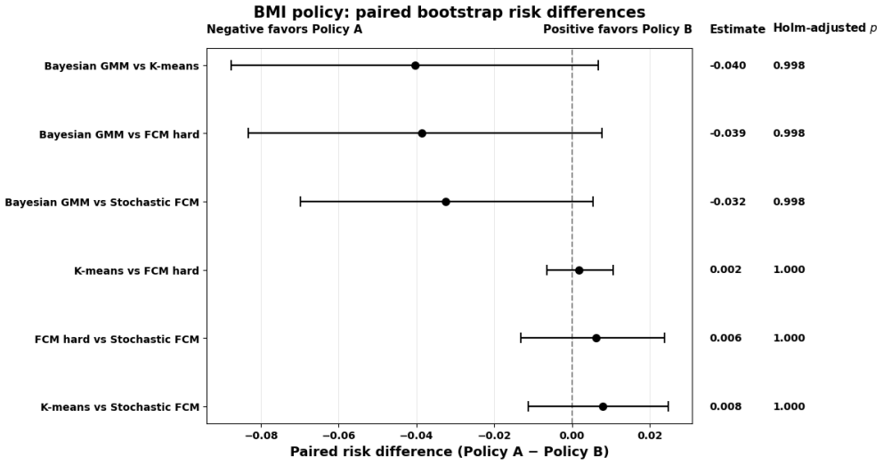
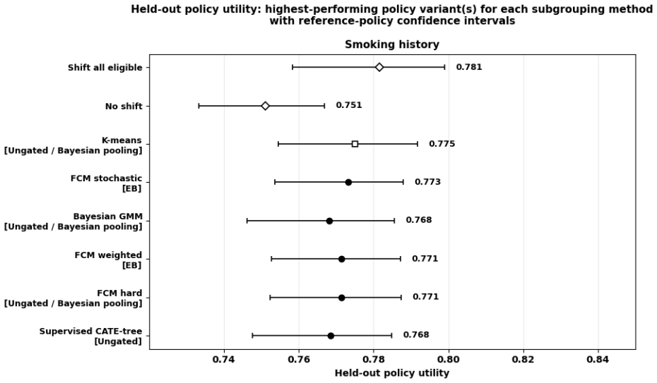
The central claim is that phenotype-first subgroups can serve as interpretable policy units in observational data, with an important qualification: method choice does not materially change estimated aggregate policy value. In representative splits, the highest ungated utility point estimates were 0.799 for the BMI policy using a Bayesian Gaussian mixture, 0.735 for the glucose policy using hard or membership-weighted fuzzy C-means, and 0.775 for the smoking-history policy using K-means; the supervised treatment-effect-guided tree never consistently beat the unsupervised methods. Paired bootstrap comparisons on the same evaluation individuals gave confidence intervals that all included zero,
What carries the argument
The load-bearing machinery is the selective one-way state-shift policy combined with an intervention-specific doubly robust estimator. For a chosen budget, each subgroup receives a shift probability between 0 and 1: fully selected clusters get 1, unselected clusters get 0, and the boundary cluster gets the fraction of its eligible members covered. The evaluated score adds a propensity-weighted residual to the outcome-regression prediction, and is averaged over the overlap-restricted held-out cohort. Subgroup ranking is driven by the discovery-side 'gain'—estimated mean benefit times eligible cluster size—computed after clustering on pre-treatment covariates only, with the cluster rule frozen
Load-bearing premise
The estimates recover true policy risk only if, conditional on the covariates chosen via causal discovery, the untreated-state outcome is independent of the adverse-state indicator (no unmeasured confounding), positivity and consistency hold, and missingness is completely at random.
What would settle it
Run the same pipeline on a semi-synthetic version of the two cohorts with known individual treatment effects generated from a hidden confounder that affects both the state and the outcome. If any method with a clearly different allocation has true utility outside the other methods' bootstrap intervals, or if estimated utilities separate by more than the paired intervals, the paper's flat-surface conclusion fails in that setting.
If this is right
- If method choice barely moves utility, then reported utility differences across algorithms should not drive deployment; decisions should weight subgroup interpretability, allocation composition, and stability across data splits.
- Effect-guided subgroup construction is not guaranteed to improve budgeted policy utility even when it improves within-group effect homogeneity.
- Safety gating is a value judgment: a conservative lower-confidence-bound gate can produce a no-shift policy, while partial pooling stays close to ungated allocation; the right choice depends on intervention risk.
- Similar estimated utility does not imply similar targeting, so policy reports should include allocation-overlap metrics, not just mean utility.
- All policy values are conditional on causal identification, so external, longitudinal, or prospective validation is required before deployment.
Where Pith is reading between the lines
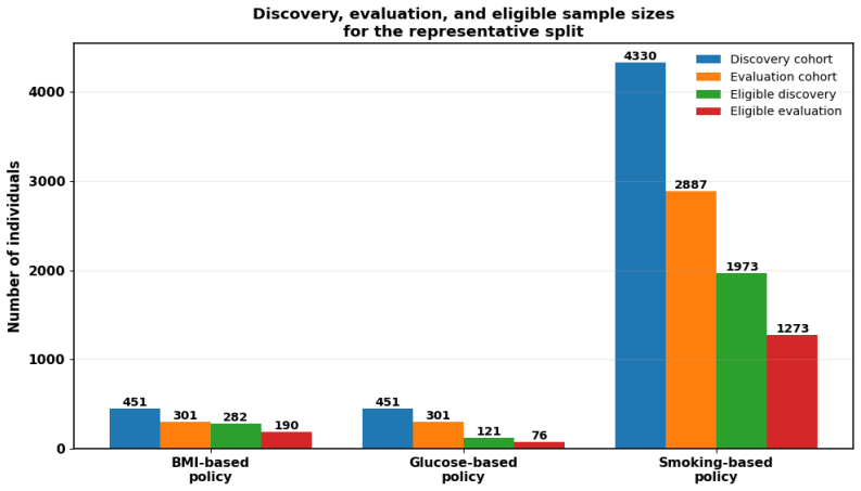
- The fixed 70% budget is generous, making most policies resemble the shift-all-eligible reference; a lower budget, such as 20-30%, would likely widen utility differences and test whether the flat policy-value surface is an artifact of the abundant capacity.
- If the flat surface persists across budgets, then the practical policy choice becomes distributional: since different algorithms select different patient sets, a decision-maker could choose among nearly equal policies using equity, clinical-profile, or implementation criteria.
- The paper conditions on one causal graph; propagating uncertainty over the discovered graph into the policy-value intervals would broaden them and further weaken any apparent method differences, which is a natural next test.
- Because the analysis uses complete cases only, informative missingness could bias all utilities; graph-aware imputation and re-running the comparisons would check whether the no-difference conclusion survives.
Editorial analysis
A structured set of objections, weighed in public.
Referee Report
Summary. The paper proposes an end-to-end framework for constructing budget-constrained, hypothetical state-shift policies from unsupervised subgroups that are defined on pre-treatment covariates, and evaluates it on PIMA (BMI and glucose contrasts) and NHANES (smoking-history contrast). The subgrouping methods compared are K-means, three FCM variants, Bayesian GMM, and a supervised CATE-tree comparator; policies are formed under ungated allocation, an Empirical Bernstein safety gate, or hierarchical Bayesian pooling. The central empirical claim is that methods with statistically indistinguishable held-out doubly robust utilities can nevertheless prioritize substantially different individuals, and that no subgrouping algorithm consistently dominates in paired bootstrap comparisons after Holm adjustment.
Significance. If the result holds, the paper makes a practically useful point: when aggregate policy utilities are flat across subgrouping algorithms, method choice should be driven by subgroup interpretability, allocation composition, and stability. The evaluation design has genuine strengths: a discovery/evaluation split, a cross-fitted doubly robust estimator (Eq. 42–44), paired bootstrap comparisons on common resamples, Holm multiplicity adjustment, multiple split seeds, and unusually explicit caveats about causal assumptions. The tables are internally consistent (utility = 1 − risk throughout), and the paper does not oversell point-estimate leaders. However, the headline claim that subgroups are constructed 'without using exposure, outcome, or estimated treatment-effect information' is weakened by an upstream causal-discovery covariate-selection step that appears to use the full dataset, and the central flat-utility conclusion is not accompanied by a sensitivity analysis for unmeasured confounding or informative missingness.
major comments (3)
- [§0.2, Algorithm 1 Step 1, Abstract] The causal-discovery-informed covariate selection appears to be performed before the discovery/evaluation split and uses the outcome variable (e.g., diabetes status, sleep disturbance) to infer the graph from which clustering and adjustment variables are chosen. The split described in §0.10 protects the clustering and ranking steps but not this upstream step. Thus the abstract's claim that subgroups are built 'without using exposure, outcome, or estimated treatment-effect information' is overstated, and the construction-to-evaluation chain is not fully non-circular. Please either re-run the CSD/domain selection using only the discovery cohort, or provide a sensitivity analysis demonstrating that the selected covariate and adjustment sets are stable under discovery-only estimation, and qualify the wording of the claim.
- [§0.5, Eqs. 40–44; Limitations] All reported utilities and the central flat-utility conclusion pass through the doubly robust estimator in Eqs. 40–44, whose identification relies on conditional exchangeability given L, positivity, consistency, and—because of complete-case analysis—MCAR. The paper explicitly acknowledges these assumptions but provides no sensitivity analysis quantifying how strong unmeasured confounding or informative missingness would need to be to change the cross-method comparisons. Since different policies place different shift probabilities on different clusters, the bias from a shared inadequate adjustment set would not be constant across policies, so the observed flat utility surface could in principle be an artifact of that shared misspecification. A concrete sensitivity analysis (e.g., E-values or latent-confounder perturbation) is needed to make the empirical claim robust.
- [§0.4.1, Eqs. 21–22] The effective-sample-size adaptation of the Empirical Bernstein bound for weighted FCM is explicitly acknowledged to be 'rather than an exact application' and is interpreted as a conservative admission score. That is a reasonable practical choice, but the earlier statement that the collection of bounds 'is intended to hold simultaneously with probability at least 1−δ' is not guaranteed under the weighted effective-sample-size modification. The paper should state clearly that the family-wise error guarantee applies only to the unweighted hard-assignment case, and that the weighted version is an approximation whose operating characteristics are not formally established.
minor comments (7)
- [§0.2] Typos and grammar: 'the figure 2 shows', 'the graph learnt', and similar informal phrasing appear; please standardize to formal journal style.
- [§0.5, Eq. 44] The augmentation term in Eq. 44 is not derived. A short derivation or an explicit statement of the relevant result in Wen et al. (2023) would help readers verify that this score is doubly robust for the selective one-way shift estimand under the stated nuisance-model conditions.
- [§0.13–0.15, Tables 3, 8, 13] The term 'utility' is used for 1 − risk, which is a risk complement rather than an economic utility. Please clarify once that no cost or benefit beyond the outcome is modeled, so 'utility' should not be read as a welfare measure.
- [Table 13] The FCM weighted EB-gated variant has a slightly higher point utility (0.7715) than the corresponding ungated policy (0.7714), which is an exception to the general statement that EB gating is always more conservative. The text describing this table should acknowledge this exception explicitly.
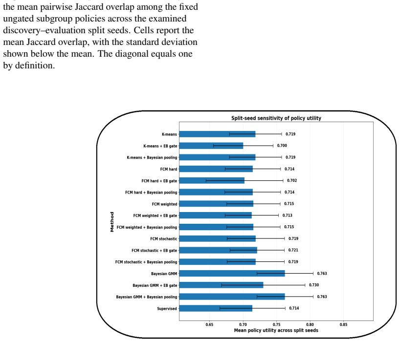
- [§0.17, Figures 13–18] The split-seed sensitivity analysis uses only four seeds. Given the small datasets and the known instability of clustering solutions, four seeds is a limited check; the paper should state that this is exploratory and not a formal stability guarantee.
- [Algorithm 1, Step 8] The random boundary-cluster selection introduces an additional source of allocation variability, but the overlap metrics are computed from realized binary selections. The paper should state whether the reported overlaps are averaged over boundary-selection seeds, and how sensitive the Jaccard values are to this random draw.
- [General] No code or detailed data-availability statement is provided. Making the analysis code and preprocessing scripts available would materially improve reproducibility, especially for the exact MCA dimension retention and the CSD ensemble construction.
Circularity Check
No significant circularity: subgroup construction is separated from benefit estimation and held-out evaluation by explicit discovery/evaluation splits.
full rationale
The paper's derivation chain is deliberately anti-circular: clustering is fit only on pre-treatment covariates in the discovery cohort (Algorithm 1, Steps 4-5), benefit scores are computed afterward and only for ranking (Step 6), and the policy is frozen before being evaluated on the held-out evaluation cohort with a separate doubly robust estimator (Steps 8-9). The evaluation utilities in Tables 3, 8, and 13 are not algebraic transforms of the discovery-side benefit scores; they are computed from out-of-sample pseudo-outcomes with cross-fitted nuisance functions. Eq. 40-45 identify the policy risk under explicit conditional exchangeability, positivity, and consistency assumptions; this is an identifying assumption, not a tautology. The paper repeatedly flags the dependence of its conclusions on the adequacy of the adjustment set and on the absence of unmeasured confounding, and it explicitly treats the causal-discovered graphs as 'potential causal structures' rather than confirmed graphs. The reuse of the authors' prior CSD procedure (ref [11]) provides the adjustment set but is not a derivation that reduces the central claim to its own input; it is an external methodological dependency that the paper discloses. The null pairwise comparisons and flat utility surface are empirical findings, not consequences of equation substitution. No step was found in which a prediction is equivalent by construction to a fitted parameter or in which the load-bearing argument reduces to a self-citation.
Axiom & Free-Parameter Ledger
free parameters (8)
- Number of clusters K =
K=3 (BMI), 4 (glucose), 6 (smoking)
- FCM fuzziness parameter m =
1.7
- Intervention budget q =
0.70
- Bayesian gate threshold π0 =
0.90
- EB gate total error δ =
0.05
- Overlap trimming α =
0.05
- Retained MCA dimensions (NHANES) =
7
- Hierarchical prior hyperparameters =
σ_μ, σ_τ, ν (weakly informative)
axioms (8)
- domain assumption Conditional exchangeability: potential outcomes under the lower-risk state are independent of observed state given the adjustment set L (no unmeasured confounding)
- domain assumption Positivity/overlap of the state probability within the adjustment set (trimmed at α=0.05)
- domain assumption Consistency and no interference of the hypothetical state shift
- domain assumption Missing Completely At Random for complete-case analysis
- domain assumption The ensemble causal-discovery graphs (data-driven + domain-augmented) identify plausible pretreatment covariates and adjustment variables
- domain assumption Benefit scores from logistic GLMs adequately approximate the state-contrast (no unmodeled nonlinear response patterns)
- ad hoc to paper Effective-sample-size adaptation of the empirical-Bernstein bound behaves as a conservative admission score
- domain assumption Hardening rules (max-membership, MAP, or stochastic sampling) map fuzzy/probabilistic clusters to operational decisions
read the original abstract
Conventional subgroup analyses can yield unstable and difficult-to-interpret conclusions, especially in observational biomedical data where each individual is observed under only one exposure state, true individual treatment effects are unavailable, and causal structure is uncertain. We investigate whether subgroups constructed from pretreatment characteristics, without using exposure, outcome, or estimated treatment-effect information, can serve as interpretable units for budget-constrained policy prioritization. We propose a framework combining causal-discovery-informed covariate selection, discovery-evaluation sample splitting, inductive unsupervised clustering, uncertainty-aware subgroup selection, and held-out doubly robust policy evaluation. We compare K-means, hard, membership-weighted, and stochastic Fuzzy C-means, Bayesian Gaussian mixture models, and a supervised causal-forest-derived CATE-tree comparator. Policies are evaluated under a 70% budget for hypothetical obesity-to-non-obesity and elevated-to-lower-glucose state shifts in the PIMA Indians Diabetes dataset and for a lifetime-smoking-history contrast in NHANES. The highest estimated ungated utilities were 0.799 for the BMI policy using Bayesian GMM, 0.735 for the glucose policy using hard or membership-weighted FCM, and 0.775 for the smoking-history policy using K-means. All paired 95% confidence intervals for policy-risk differences included zero, and no comparison remained statistically significant after Holm adjustment. Bayesian pooling generally preserved ungated allocations, whereas Empirical Bernstein gating was more conservative. Policies with similar estimated utility could nevertheless prioritize different individuals. The findings should be interpreted as assumption-dependent decision-support evidence for hypothetical state contrasts rather than proof of intervention benefit.
Figures






Reference graph
Works this paper leans on
-
[1]
& Imbens, G
Athey, S. & Imbens, G. Recursive partitioning for heterogeneous causal effects.Proc. Natl. Acad. Sci.113, 7353–7360 (2016)
2016
-
[2]
& Athey, S
Wager, S. & Athey, S. Estimation and inference of heterogeneous treatment effects using random forests.J. Am. Stat. Assoc.113, 1228–1242 (2018). 3.Holland, P. W. Statistics and causal inference.J. Am. statistical Assoc.81, 945–960 (1986). 4.Hill, J. L. Bayesian nonparametric modeling for causal inference.J. Comput. Graph. Stat.20, 217–240 (2011)
2018
-
[5]
Shalit, U., Johansson, F. D. & Sontag, D. Estimating individual treatment effect: generalization bounds and algorithms. InInternational conference on machine learning, 3076–3085 (PMLR, 2017)
2017
-
[6]
R., Sekhon, J
Künzel, S. R., Sekhon, J. S., Bickel, P. J. & Yu, B. Metalearners for estimating heterogeneous treatment effects using machine learning.Proc. national academy sciences116, 4156–4165 (2019)
2019
-
[7]
C., Taylor, J
Foster, J. C., Taylor, J. M. & Ruberg, S. J. Subgroup identification from randomized clinical trial data.Stat. medicine30, 2867–2880 (2011)
2011
-
[8]
Lindeman, N. I.et al.Updated molecular testing guideline for the selection of lung cancer patients for treatment with targeted tyrosine kinase inhibitors: guideline from the college of american pathologists, the international association for the study of lung cancer, and the association for molecular pathology.Arch. pathology & laboratory medicine142, 321...
2018
-
[9]
Sepulveda, A. R.et al.Molecular biomarkers for the evaluation of colorectal cancer: guideline from the american society for clinical pathology, college of american pathologists, association for molecular pathology, and american society of clinical oncology.Am. journal clinical pathology147, 221–260 (2017)
2017
-
[10]
C., Louis, T
Henderson, N. C., Louis, T. A., Wang, C. & Varadhan, R. Bayesian analysis of heterogeneous treatment effects for patient-centered outcomes research.Heal. Serv. Outcomes Res. Methodol.16, 213–233 (2016)
2016
-
[11]
Acharya, V ., Yener, B., Fields, M. C. & Marcuse, L. V . Understanding the impact of epilepsy and depression on sleep disorder: Beyond associations. In2025 IEEE EMBS International Conference on Biomedical and Health Informatics (BHI), 1–7 (IEEE, 2025)
2025
-
[12]
M., Rothwell, P
Kent, D. M., Rothwell, P. M., Ioannidis, J. P., Altman, D. G. & Hayward, R. A. Assessing and reporting heterogeneity in treatment effects in clinical trials: a proposal.Trials11, 85 (2010)
2010
-
[13]
J., Hayward, R
Dahabreh, I. J., Hayward, R. & Kent, D. M. Using group data to treat individuals: understanding heterogeneous treatment effects in the age of precision medicine and patient-centred evidence.Int. journal epidemiology45, 2184–2193 (2016)
2016
-
[14]
& Fernandez-Val, I
Chernozhukov, V ., Demirer, M., Duflo, E. & Fernandez-Val, I. Generic machine learning inference on heterogeneous treatment effects in randomized experiments, with an application to immunization in india. Tech. Rep., National Bureau of Economic Research (2018)
2018
-
[15]
& Kennedy, E
Kim, K., Kim, J. & Kennedy, E. H. Causal k-means clustering.J. Royal Stat. Soc. Ser. B: Stat. Methodol.qkag068 (2026)
2026
-
[16]
& Yang, S
Wang, Z., Ayer, T. & Yang, S. Causal clustering for conditional average treatment effects estimation and subgroup discovery. In2025 IEEE EMBS International Conference on Biomedical and Health Informatics (BHI), 1–11 (IEEE, 2025)
2025
-
[17]
Bellavia, A.et al.Unsupervised clustering approach to assess heterogeneity of treatment effects across patient phenotypes in randomized clinical trials.Contemp. Clin. Trials148, 107778 (2025)
2025
-
[18]
Sinha, P.et al.Comparison of machine learning clustering algorithms for detecting heterogeneity of treatment effect in acute respiratory distress syndrome: a secondary analysis of three randomised controlled trials.EBioMedicine74(2021)
2021
-
[19]
K.et al.Identification of acute kidney injury subphenotypes with differing molecular signatures and responses to vasopressin therapy.Am
Bhatraju, P. K.et al.Identification of acute kidney injury subphenotypes with differing molecular signatures and responses to vasopressin therapy.Am. journal respiratory critical care medicine199, 863–872 (2019)
2019
-
[20]
Zampieri, F. G.et al.Heterogeneous effects of alveolar recruitment in acute respiratory distress syndrome: a machine learning reanalysis of the alveolar recruitment for acute respiratory distress syndrome trial.Br. journal anaesthesia123, 88–95 (2019)
2019
-
[21]
& Meir, R
Derbeko, P., El-Yaniv, R. & Meir, R. Explicit learning curves for transduction and application to clustering and compression algorithms.J. Artif. Intell. Res.22, 117–142 (2004)
2004
-
[22]
& Terami, A
Miyamoto, S. & Terami, A. Inductive vs. transductive clustering using kernel functions and pairwise constraints. In2011 11th International Conference on Intelligent Systems Design and Applications, 1258–1264 (IEEE, 2011). 38/41
2011
-
[23]
neural information processing systems16(2003)
Bengio, Y .et al.Out-of-sample extensions for lle, isomap, mds, eigenmaps, and spectral clustering.Adv. neural information processing systems16(2003)
2003
-
[24]
& Al-Khassaweneh, M
Stewart, G. & Al-Khassaweneh, M. An implementation of the hdbscan* clustering algorithm.Appl. Sci.12, 2405 (2022). 25.Nie, X. & Wager, S. Quasi-oracle estimation of heterogeneous treatment effects.Biometrika108, 299–319 (2021)
2022
-
[26]
Hahn, P. R., Murray, J. S. & Carvalho, C. M. Bayesian regression tree models for causal inference: Regularization, confounding, and heterogeneous effects (with discussion).Bayesian Analysis15, 965–1056 (2020). 27.Souto, H. G. & Neto, F. L. K-fold causal bart for cate estimation.arXiv preprint arXiv:2409.05665(2024)
Pith/arXiv arXiv 2020
-
[28]
& Van Der Laan, M
Bibaut, A., Malenica, I., Vlassis, N. & Van Der Laan, M. More efficient off-policy evaluation through regularized targeted learning. InInternational Conference on Machine Learning, 654–663 (PMLR, 2019). 29.Athey, S. & Wager, S. Policy learning with observational data.Econometrica89, 133–161 (2021)
2019
-
[30]
Bang, H. & Robins, J. M. Doubly robust estimation in missing data and causal inference models.Biometrics61, 962–973 (2005). 31.Dudík, M., Langford, J. & Li, L. Doubly robust policy evaluation and learning.arXiv preprint arXiv:1103.4601(2011)
Pith/arXiv arXiv 2005
-
[32]
& Tetenov, A
Kitagawa, T. & Tetenov, A. Who should be treated? empirical welfare maximization methods for treatment choice. Econometrica86, 591–616 (2018)
2018
-
[33]
& Zhou, Z
Kallus, N., Mao, X., Wang, K. & Zhou, Z. Doubly robust distributionally robust off-policy evaluation and learning. In International Conference on Machine Learning, 10598–10632 (PMLR, 2022)
2022
-
[34]
& Ghavamzadeh, M
Thomas, P., Theocharous, G. & Ghavamzadeh, M. High-confidence off-policy evaluation. InProceedings of the AAAI Conference on Artificial Intelligence, vol. 29 (2015)
2015
-
[35]
& Wang, Z
Jin, Y ., Ren, Z., Yang, Z. & Wang, Z. Policy learning “without” overlap: Pessimism and generalized empirical bernstein’s inequality.The Annals Stat.53, 1483–1512 (2025)
2025
-
[36]
F., Cole, S
Schisterman, E. F., Cole, S. R. & Platt, R. W. Overadjustment bias and unnecessary adjustment in epidemiologic studies. Epidemiology20, 488–495 (2009). 37.VanderWeele, T. J. Principles of confounder selection: Tj vanderweele.Eur. journal epidemiology34, 211–219 (2019)
2009
-
[38]
Hernán, M. A. & Taubman, S. L. Does obesity shorten life? the importance of well-defined interventions to answer causal questions.Int. journal obesity32, S8–S14 (2008)
2008
-
[39]
& Shen, Q
Su, P., Shang, C. & Shen, Q. A hierarchical fuzzy cluster ensemble approach and its application to big data clustering.J. Intell. & Fuzzy Syst.28, 2409–2421 (2015)
2015
-
[40]
W., Everhart, J
Smith, J. W., Everhart, J. E., Dickson, W. C., Knowler, W. C. & Johannes, R. S. Using the adap learning algorithm to forecast the onset of diabetes mellitus. InProceedings of the annual symposium on computer application in medical care, 261 (1988). 41.Greenacre, M. J.Theory and Applications of Correspondence Analysis(Academic Press, 1984)
1988
-
[42]
Greenacre, M. J. & Blasius, J. (eds.)Multiple Correspondence Analysis and Related Methods(Chapman and Hall/CRC, 2006). 43.Abdi, H. & Valentin, D. Multiple correspondence analysis.Encycl. Meas. Stat.(2007)
2006
-
[44]
& Meulman, J
Lombardo, R. & Meulman, J. J. Multiple correspondence analysis via polynomial transformations of ordered categorical variables.J. Classif.27, 191–210 (2010)
2010
-
[45]
& Greenacre, M
Nenadi´c, O. & Greenacre, M. Correspondence analysis in r, with two- and three-dimensional graphics: The ca package.J. Stat. Softw.20, 1–13 (2007)
2007
-
[46]
Florensa, D.et al.Use of multiple correspondence analysis and k-means to explore associations between risk factors and likelihood of colorectal cancer: Cross-sectional study.J. Med. Internet Res.24, e29056 (2022)
2022
-
[47]
S., Santos, N
Costa, P. S., Santos, N. C., Cunha, P., Cotter, J. & Sousa, N. The use of multiple correspondence analysis to explore associations between categories of qualitative variables in healthy ageing.J. aging research2013, 302163 (2013)
2013
-
[48]
clinical epidemiology63, 638–646 (2010)
Sourial, N.et al.Correspondence analysis is a useful tool to uncover the relationships among categorical variables.J. clinical epidemiology63, 638–646 (2010)
2010
-
[49]
Violán, C.et al.Multimorbidity patterns with k-means nonhierarchical cluster analysis.BMC family practice19, 108 (2018). 39/41
2018
-
[50]
Hwang, H., Dillon, W. R. & Takane, Y . An extension of multiple correspondence analysis for identifying heterogeneous subgroups of respondents.Psychometrika71, 161–171 (2006)
2006
-
[51]
& van der Schaar, M
Kyono, T., Zhang, Y ., Bellot, A. & van der Schaar, M. Miracle: Causally-aware imputation via learning missing data mechanisms. InConference on Neural Information Processing Systems(NeurIPS) 2021(2021)
2021
-
[52]
An anytime algorithm for causal inference
Spirtes, P. An anytime algorithm for causal inference. InInternational Workshop on Artificial Intelligence and Statistics, 278–285 (PMLR, 2001)
2001
-
[53]
& Xing, E
Zheng, X., Dan, C., Aragam, B., Ravikumar, P. & Xing, E. Learning sparse nonparametric dags. InInternational conference on artificial intelligence and statistics, 3414–3425 (Pmlr, 2020)
2020
-
[54]
& Textor, J
Ankan, A. & Textor, J. A simple unified approach to testing high-dimensional conditional independences for categorical and ordinal data. InProceedings of the AAAI Conference on Artificial Intelligence, vol. 37, 12180–12188 (2023)
2023
-
[55]
M., Peters, J
Hoyer, P., Janzing, D., Mooij, J. M., Peters, J. & Schölkopf, B. Nonlinear causal discovery with additive noise models. Adv. neural information processing systems21(2008)
2008
-
[56]
cardiovascular medicine9, 939103 (2022)
Cheng, W.et al.Age-related changes in the risk of high blood pressure.Front. cardiovascular medicine9, 939103 (2022)
2022
-
[57]
journal endocrinology175, R231–R245 (2016)
Li, P.et al.Mechanisms in endocrinology: parity and risk of type 2 diabetes: a systematic review and dose-response meta-analysis.Eur. journal endocrinology175, R231–R245 (2016)
2016
-
[58]
Ruiz-Alejos, A.et al.Skinfold thickness and the incidence of type 2 diabetes mellitus and hypertension: an analysis of the peru migrant study.Public health nutrition23, 63–71 (2020)
2020
-
[59]
A., Anderson, S
Emdin, C. A., Anderson, S. G., Woodward, M. & Rahimi, K. Usual blood pressure and risk of new-onset diabetes: evidence from 4.1 million adults and a meta-analysis of prospective studies.J. Am. Coll. Cardiol.66, 1552–1562 (2015)
2015
-
[60]
K., Lee, H
Fazeli, P. K., Lee, H. & Steinhauser, M. L. Aging is a powerful risk factor for type 2 diabetes mellitus independent of body mass index.Gerontology66, 209–210 (2020)
2020
-
[61]
& Glymour, C
Spirtes, P. & Glymour, C. An algorithm for fast recovery of sparse causal graphs.Soc. science computer review9, 62–72 (1991)
1991
-
[62]
Wang, R. & Peng, J. Learning directed acyclic graphs via bootstrap aggregating.arXiv preprint arXiv:1406.2098(2014)
Pith/arXiv arXiv 2098
-
[63]
& Glymour, C
Ramsey, J., Glymour, M., Sanchez-Romero, R. & Glymour, C. A million variables and more: the fast greedy equivalence search algorithm for learning high-dimensional graphical causal models, with an application to functional magnetic resonance images.Int. journal data science analytics3, 121–129 (2017)
2017
-
[64]
Some methods for classification and analysis of multivariate observations
MacQueen, J. Some methods for classification and analysis of multivariate observations. InProceedings of the Fifth Berkeley Symposium on Mathematical Statistics and Probability, vol. 1, 281–297 (University of California Press, 1967)
1967
-
[65]
Dunn, J. C. A fuzzy relative of the isodata process and its use in detecting compact well-separated clusters.J. Cybern.3, 32–57 (1973). 66.Bezdek, J. C.Pattern Recognition with Fuzzy Objective Function Algorithms(Plenum Press, New York, 1981)
1973
-
[67]
Bezdek, J. C., Ehrlich, R. & Full, W. Fcm: The fuzzy c-means clustering algorithm.Comput. & Geosci.10, 191–203, DOI: 10.1016/0098-3004(84)90020-7 (1984). 68.Wu, K.-L. Analysis of parameter selections for fuzzy c-means.Pattern Recognit.45, 407–415 (2012)
-
[69]
Schwämmle, V . & Jensen, O. N. A simple and fast method to determine the parameters for fuzzy c–means cluster analysis. Bioinformatics26, 2841–2848 (2010). 70.Wu, Q., Zhu, Z. & Zhang, A. R. Statistical inference for fuzzy clustering (2026). 2601.02656
arXiv 2010
-
[71]
Zhao, Y .et al.Mapping phenotypic heterogeneity and cardiometabolic risk in obesity using a tree-based dimensionality reduction framework.J. Transl. Medicine24, 401 (2026)
2026
-
[72]
Rasmussen, C. E. The infinite gaussian mixture model. InAdvances in Neural Information Processing Systems, vol. 12, 554–560 (MIT Press, 2000). 73.Blei, D. M. & Jordan, M. I. Variational inference for dirichlet process mixtures.Bayesian Analysis1, 121–144 (2006)
2000
-
[74]
Maurer, A. & Pontil, M. Empirical bernstein bounds and sample variance penalization.arXiv preprint arXiv:0907.3740 (2009)
Pith/arXiv arXiv 2009
-
[75]
& Yajima, M
Gelman, A., Hill, J. & Yajima, M. Why we (usually) don’t have to worry about multiple comparisons.J. research on educational effectiveness5, 189–211 (2012). 40/41 76.Gelman, A. Prior distributions for variance parameters in hierarchical models.Bayesian Analysis1, 515–533 (2006)
2012
-
[77]
Polson, N. G. & Scott, J. G. On the half-cauchy prior for a global scale parameter.Bayesian Analysis7, 887–902 (2012). 78.Morris, C. N. Parametric empirical bayes inference: Theory and applications.J. Am. Stat. Assoc.78, 47–55 (1983)
2012
-
[79]
Wen, L., Marcus, J. L. & Young, J. G. Intervention treatment distributions that depend on the observed treatment process and model double robustness in causal survival analysis.Stat. methods medical research32, 509–523 (2023). 80.Purnell, J. Q. Definitions, classification, and epidemiology of obesity (2015). 81.Bansal, N. Prediabetes diagnosis and treatme...
2023
-
[82]
W., Ware, J
Wang, R., Lagakos, S. W., Ware, J. H., Hunter, D. J. & Drazen, J. M. Statistics in medicine—reporting of subgroup analyses in clinical trials.New Engl. J. Medicine357, 2189–2194 (2007). 83.Hall, P. & Wilson, S. R. Two guidelines for bootstrap hypothesis testing.Biometrics757–762 (1991). 84.Holm, S. A simple sequentially rejective multiple test procedure.S...
2007
-
[86]
& Gensler, H
Aickin, M. & Gensler, H. Adjusting for multiple testing when reporting research results: the bonferroni vs holm methods. Am. journal public health86, 726–728 (1996)
1996
-
[87]
Étude comparative de la distribution florale dans une portion des alpes et des jura.Bull Soc Vaudoise Sci Nat 37, 547–579 (1901)
Jaccard, P. Étude comparative de la distribution florale dans une portion des alpes et des jura.Bull Soc Vaudoise Sci Nat 37, 547–579 (1901)
1901
-
[88]
Powers, D. M. Evaluation: from precision, recall and f-measure to roc, informedness, markedness and correlation.arXiv preprint arXiv:2010.16061(2020)
Pith/arXiv arXiv 2010
-
[89]
& Boulesteix, A.-L
Ullmann, T., Hennig, C. & Boulesteix, A.-L. Validation of cluster analysis results on validation data: A systematic framework.Wiley Interdiscip. Rev. Data Min. Knowl. Discov.12, e1444 (2022)
2022
-
[90]
C., Taylor, J
Foster, J. C., Taylor, J. M. & Ruberg, S. J. Subgroup identification from randomized clinical trial data.Stat. medicine30, 2867–2880 (2011). 91.Pedregosa, F.et al.Scikit-learn: Machine learning in python.J. machine Learn. research12, 2825–2830 (2011). 92.Warner, J.et al.Jdwarner/scikit-fuzzy: Scikit-fuzzy 0.5. 0.Zenodo(2024). 93.Halford, M. Prince
2011
-
[94]
https://github.com/py-why/EconML (2019)
Battocchi, K.et al.EconML: A Python Package for ML-Based Heterogeneous Treatment Effects Estimation. https://github.com/py-why/EconML (2019). Version 0.x
2019
-
[95]
Sci.9, DOI: 10.7717/peerj-cs.1516 (2023)
Abril-Pla, O.et al.PyMC: A modern and comprehensive probabilistic programming framework in Python.PeerJ Comput. Sci.9, DOI: 10.7717/peerj-cs.1516 (2023). 96.Zheng, Y .et al.Causal-learn: Causal discovery in python.J. Mach. Learn. Res.25, 1–8 (2024). 97.Ankan, A. & Textor, J. Pgmpy: a python toolkit for bayesian networks.J. Mach. Learn. Res.25, 1–8 (2024)....
-
[99]
Goodman, L. A. Exploratory latent structure analysis using both identifiable and unidentifiable models.Biometrika61, 215–231 (1974)
1974
-
[100]
Extensions to the k-means algorithm for clustering large data sets with categorical values.Data mining knowledge discovery2, 283–304 (1998)
Huang, Z. Extensions to the k-means algorithm for clustering large data sets with categorical values.Data mining knowledge discovery2, 283–304 (1998)
1998
-
[101]
Jama295, 1152–1160 (2006)
Piaggio, G.et al.Reporting of noninferiority and equivalence randomized trials: an extension of the consort statement. Jama295, 1152–1160 (2006)
2006
-
[102]
M., D HULING, J
Maronge, J. M., D HULING, J. & Chen, G. A reluctant additive model framework for interpretable nonlinear individualized treatment rules.The annals applied statistics17, 3384 (2023)
2023
-
[103]
& Veeramachaneni, K
Zytek, A., Arnaldo, I., Liu, D., Berti-Equille, L. & Veeramachaneni, K. The need for interpretable features: Motivation and taxonomy.ACM SIGKDD Explor. Newsl.24, 1–13 (2022)
2022
-
[104]
& Vichi, M
Fordellone, M. & Vichi, M. Multiple correspondence k-means: simultaneous versus sequential approach for dimension reduction and clustering. InData Science and Social Research: Epistemology, Methods, Technology and Applications, 81–95 (Springer, 2017)
2017
-
[105]
& Livny, M
Zhang, T., Ramakrishnan, R. & Livny, M. Birch: an efficient data clustering method for very large databases.ACM sigmod record25, 103–114 (1996). 41/41
1996
discussion (0)
Sign in with ORCID, Apple, or X to comment. Anyone can read and Pith papers without signing in.