REVIEW 3 major objections 5 minor 2 cited by
Six-wave mixing lifts Rydberg receiver bandwidth to 7.2 MHz in simulation
Reviewed by Pith at T0; open to challenge. T0 means a machine referee read the full paper against a public rubric. the ladder, T0–T4 →
A six-wave-mixing Rydberg receiver is modeled as a two-pole low-pass RF-to-optical transducer, claimed to reach ~7.2 MHz baseband bandwidth versus ~0.66 MHz for EIT, with a tunable bandwidth-linearity trade-off.
T0 review reviewed 2026-08-02 challenge →
load-bearing objection Useful modeling framework, but the headline bandwidth claim is contradicted by the paper's own parameters: the two-pole model gives about 2 MHz, not the reported 7-10 MHz. the 3 major comments →
Wideband Quantum Transduction for Rydberg Atomic Receivers Using Six-Wave Mixing
The pith
A machine-rendered reading of the paper's core claim, the machinery that carries it, and where it could break.
The reading
Core claim
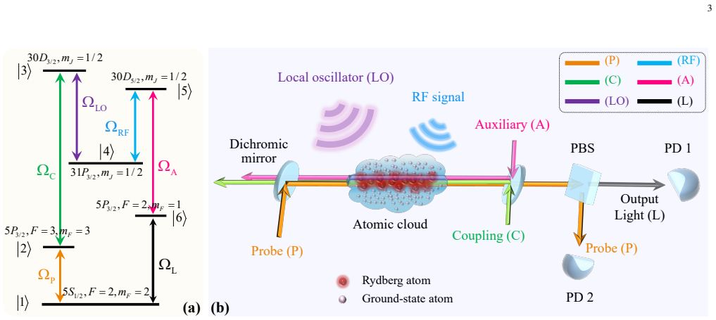
The central discovery, stated in the authors' own terms, is an explicit input-output baseband model: the detected six-wave-mixing coherence ρ61(ω) equals (i/2)^5 ΩPΩCΩLO/(D2D3D4) times ΩA*ΩRF(ω)/(D5(ω)D6(ω)+|ΩA|^2/4), from which the fifth-order polarization and finally the photocurrent are derived. Because the analysis frequencies are small compared with the detunings and dephasing of levels |2>, |3>, |4>, only D5 and D6 retain frequency dependence, so the RF-to-optical link becomes a second-order low-pass with a closed-form 3-dB bandwidth. Numerical solution of the full master equation gives f3dB≈7.2 MHz for SWM versus 0.66 MHz for EIT under identical optical drives, with comparable sensiti
What carries the argument
The load-bearing object is the closed six-wave-mixing loop |1>→|2>→|3>→|4>→|5>→|6>→|1>, driven by probe, coupling, local-oscillator, RF, and auxiliary fields, which emits the output light field whose envelope carries the RF signal. The analytical machinery is the reduced-order two-pole low-pass model: after adiabatic elimination of the intermediate coherences D2, D3, D4, the denominator factors as D5(ω)D6(ω)+|ΩA|^2/4 = (s−λ+)(s−λ−), so the response is governed by two effective decay rates γ+ and γ−. The auxiliary-field Rabi frequency ΩA sets the splitting between those poles and thereby acts as the bandwidth knob that the paper tunes to reach roughly 7 MHz.
Load-bearing premise
The load-bearing premise is that the single-photon detunings of levels |3> and |4> are large enough that the intermediate coherences D3 and D4 have no frequency dependence up to the claimed 7 MHz bandwidth; the paper states this assumption immediately after Eq. 8 but never gives the detuning values, even though γ31/2π=50 kHz and γ41/2π=80 kHz are much smaller than the claimed bandwidth.
What would settle it
Run the described cold-87Rb experiment with the paper's Rabi frequencies, sweep a weak RF modulation tone from DC to 20 MHz, and measure the power at the optical beat output. If the 3-dB roll-off occurs below roughly 1 MHz, near the γ31 or γ41 dephasing values, rather than near the predicted 7.2 MHz, the frequency independence of the intermediate coherences is violated and the two-pole model is not the operative bandwidth limit.
If this is right
- The SWM receiver can carry baseband modulation to around 7 MHz at a sensitivity comparable to the EIT receiver, removing the hundreds-of-kHz ceiling that limits current Rydberg receivers.
- The auxiliary-field Rabi frequency is a clean engineering control: increasing it widens the 3-dB bandwidth and, over a broad range, also improves the IIP3, so bandwidth and linearity can be traded smoothly rather than against each other.
- P1dB and IIP3 calculated from the third-order atomic response give standard communication metrics (SWM IIP3 ≈7.31 MHz, EIT ≈12.71 MHz), making the quantum transducer comparable to an RF front-end for system design.
- The closed-form bandwidth formula and the validity range of the two-pole approximation let an engineer choose operating points analytically, avoiding full master-equation numerics for initial design.
- At high LO dressing the EIT configuration develops a resonant rather than strict low-pass response, so the fair use of EIT is narrowband, channelized links, while SWM is suited to wideband multicarrier operation.
Where Pith is reading between the lines
- A direct consequence the authors leave implicit is that the bandwidth ceiling is set by the dephasing of the two highest Rydberg levels: using longer-lived Rydberg states or reducing linewidths should push f3dB beyond 7 MHz, and the same two-pole formula would predict where it lands.
- The model's prediction that IIP3 rises with ΩA is testable in a two-tone cold-atom experiment before power-broadening effects appear; if instead IIP3 falls, the assumed dominance of the SWM path over competing distortion paths would need revision.
- Because the sensitivity drop at high baseband frequencies is caused by falling conversion gain rather than rising intrinsic noise, an electronic equalizer matching the two-pole roll-off could in principle recover a flat noise-equivalent field over the whole 7 MHz band.
- For realistic wideband wireless links, SWM's lower IIP3 relative to EIT implies a trade-off between instantaneous bandwidth and tolerance to blockers; the paper's complementary view suggests a hybrid receiver that switches between SWM and EIT modes depending on channel occupancy.
Editorial analysis
A structured set of objections, weighed in public.
Referee Report
Summary. The paper proposes a six-wave-mixing (SWM) Rydberg atomic receiver as a wideband RF-to-optical quantum transducer. It derives a baseband input–output model from a six-level master equation, reduces the frequency-selective response to a two-pole low-pass filter, and derives closed-form expressions for the 3-dB bandwidth, P1dB, and IIP3. Numerical simulations with QuTiP are used to claim f3dB≈7.2 MHz for SWM versus ≈0.66 MHz for EIT, with the auxiliary field Rabi frequency ΩA as a tunable bandwidth knob. The paper concludes that SWM provides a broader, more tunable, and more benign bandwidth–linearity trade-off than EIT.
Significance. If the two-pole model were valid for the operating parameters, the paper would be a useful contribution: it proposes a compact input–output model, closed-form bandwidth expressions, and maps standard RF linearity metrics onto atomic parameters, backed by extensive QuTiP simulations. The paper correctly identifies the need for communication-oriented bandwidth/linearity metrics and offers a plausible modeling framework. However, the central analytic explanation is not substantiated by the reported simulations, and the paper's own parameters violate the assumptions of its derived bandwidth formula. The claimed order-of-magnitude low-pass bandwidth enhancement and the 'strict low-pass' behavior are therefore unsupported.
major comments (3)
- [Sec. III-A, Eqs. (27)-(32)] The derivation of the closed-form bandwidth (32) assumes real poles, which requires ΩA<|γ51−γ61| as stated after Eq. (27). The simulation parameters in Sec. IV-A are ΩA/2π=6.2 MHz, γ51/2π=129 kHz, γ61/2π=6.1 MHz, so ΩA > |γ51−γ61| = 5.971 MHz. Hence the poles in Eq. (27) are complex, Eq. (29) does not hold, and Eq. (32) is not applicable. Evaluating the equal-rate formula (34) with the average decay rate gives f3dB≈0.644(γ51+γ61)/(4π)≈2.0 MHz, about 3.6 times smaller than the reported 7.2 MHz. The simulated 7.2 MHz therefore comes from an underdamped resonance, not from the monotonic two-pole low-pass model claimed in the abstract. This is a load-bearing inconsistency: the central analytical explanation of the bandwidth enhancement is contradicted by the paper's own parameters.
- [Sec. II-B after Eq. (8); Sec. IV-A parameters] The reduction to two poles neglects the ω-dependence in D2, D3, D4 on the grounds that ω is much smaller than the optical detunings and dephasing rates. But the listed intermediate-state dephasing rates are γ31/2π=50 kHz and γ41/2π=80 kHz, while the claimed bandwidth is 7.2 MHz. For analysis frequencies up to 7.2 MHz, D3(ω) and D4(ω) change substantially unless the single-photon detunings Δ3 and Δ4 are several MHz or larger. The paper never states Δ3 and Δ4, so it is impossible to verify the approximation. If these detunings are not large, the intermediate levels would introduce additional poles near 50–80 kHz, making the two-pole model inaccurate over the claimed bandwidth. The authors should specify the detunings and provide a quantitative validity check (e.g., compare the full model and the two-pole approximation) across the reported frequency range.
- [Sec. IV-B, Fig. 4 and Fig. 5] The paper defines f3dB as the frequency where |H(ω)| first drops to |H(0)|/√2. For the SWM parameters with complex poles, the transfer function is underdamped and the magnitude response is not monotonic. The reported f3dB≈7.2 MHz is therefore the high-frequency −3 dB crossing of a resonance peak, not the 3-dB bandwidth of a low-pass response. The paper itself acknowledges in Sec. IV-C2 (discussion of Fig. 11(a)) that for the EIT scheme at large ΩLO 'the spectral maximum shifts from DC to a finite frequency' and that the 'broadened bandwidth no longer reflects the effective baseband bandwidth.' The same caveat applies to the SWM simulation, so the comparison in Fig. 4 does not support the abstract's claim of a 'strict low-pass condition' or an order-of-magnitude low-pass bandwidth enhancement.
minor comments (5)
- [Sec. I, Contributions] Typo: 'compelx' should be 'complex'.
- [Sec. IV-C2] The text refers to 'the dashed curve in Fig. 8(a)' while describing the EIT bandwidth curve; the correct reference appears to be Fig. 11(a).
- [Sec. IV-B3] The sentence 'This trend is not only due to an intrinsic increase of these noise sources themselves, but rather attributes to the NEF tot with frequency' is garbled; it should say '...but rather is attributed to the frequency dependence of NEF_tot.'
- [Sec. III-C1, Eq. (53)] α(ω) is defined as the real part of H3(ω)/H1(ω), and the derivation assumes the imaginary part is negligible for the gain compression. This should be justified, or the analysis should use the magnitude of the ratio.
- [Fig. 2 and Sec. IV-B1] The text equates the FWHM of the normalized amplitude with the 3-dB power bandwidth. This equality holds only for symmetric lineshapes; a brief justification for the SWM lineshape would help.
Circularity Check
No significant circularity: the two-pole analysis and the 7.2 MHz simulation are independent derivations from the same master equation; noted discrepancies are consistency/correctness issues, not circularity.
full rationale
The derivation chain is not circular. The baseband transfer function (24) and the two-pole reduction (25)-(27) are derived from the Lindblad master equation (4) with dephasing rates and Rabi frequencies taken from external references [27],[28]; no parameter is fitted to the claimed 7.2 MHz bandwidth. The closed-form 3-dB expressions (32)-(36) are algebraic consequences of the reduced transfer function. The simulation in Sec. IV solves the same master equation, so it serves as an internal consistency check rather than an external falsification, but the paper does not present the simulation as experimental validation. The only self-citations ([7]) supply the BBR noise model and noise-budget framework for the secondary sensitivity analysis; the central bandwidth result does not depend on this citation, and the cited model is a standard physics input (Callen-Welton law), not an unverified theorem forcing the conclusion. The approximation that D2,D3,D4 are ω-independent may be questionable given the stated dephasing rates, and the 'strict low-pass condition' may be violated by the paper's own parameters; however, these are correctness/consistency concerns, not circularity in the sense of a prediction reducing to its inputs by construction.
Axiom & Free-Parameter Ledger
free parameters (5)
- γ51 coherence dephasing rate =
2π×129 kHz
- γ61 coherence dephasing rate =
2π×6.1 MHz
- ΩA auxiliary Rabi frequency =
2π×6.2 MHz
- Intermediate single-photon detunings Δ2, Δ3, Δ4 =
not specified
- ΩLO local-oscillator Rabi frequency =
2π×1.4 MHz
axioms (6)
- standard math Rotating-wave approximation and Markovian Lindblad master equation describe the six-level atomic dynamics.
- domain assumption Cold 87Rb cloud: Doppler broadening, velocity averaging, and collision/pressure broadening are negligible.
- domain assumption Weak RF signal: response is linear, so ρ61 is first order in ΩRF and higher-order coherences can be neglected.
- domain assumption Intermediate levels |2>, |3>, |4> respond instantly: D2,D3,D4 are ω-independent over the band.
- domain assumption Plane-wave 1D propagation with effective interaction length L_eff describes the output field.
- domain assumption Photodetection is a linear heterodyne beat between the probe and the generated field.
Cite this review
Pith. "Pith review of Wideband Quantum Transduction for Rydberg Atomic Receivers Using Six-Wave Mixing." pith.science (2026). https://pith.science/paper/D2Y6K5BJ
@misc{pith2026260213955,
  author       = {Pith},
  title        = {Pith review of: Wideband Quantum Transduction for Rydberg Atomic Receivers Using Six-Wave Mixing},
  year         = {2026},
  howpublished = {\url{https://pith.science/paper/D2Y6K5BJ}},
  note         = {Machine review of arXiv:2602.13955}
}
read the original abstract
This paper investigates a six-wave mixing (SWM)-based Rydberg atomic receiver as a wideband radio frequency (RF)-to-optical quantum transducer. Specifically, we develop an explicit baseband input-output model that bridges the RF-induced atomic coherence to the detected optical readout. Based on the exact detected SWM response, we develop a reduced-order closed-form two-pole low-pass approximation under the near-resonant weak-signal of interest, which provides an analytical insight into how the 3-dB bandwidth is manipulated by the dressed higher-level atomic dynamics and optical/RF parameters. The validity range of this approximation is then quantified to clarify the operating conditions under which this reduced-order model accurately represents the exact SWM response. We further characterize the linear dynamic range by employing the 1-dB compression point (P1dB) and the input-referred third-order intercept point (IIP3), unveiling a communication-compatible characterization of the bandwidth-sensitivity-linearity trade-off. Extensive simulation results demonstrate that SWM can achieve a 3-dB bandwidth of approximately 10 MHz while maintaining favorable linearity and sensitivity under the strict low-pass condition. The comparison with the EIT regime indicates that the two schemes should be treated as complementary rather than universally ordered. From an engineering perspective, the preferred SWM operating region is therefore not the one with the largest bandwidth, but the one that simultaneously provides a large bandwidth, acceptable sensitivity, favorable linearity, and low-pass regularity.
Figures


Forward citations
Cited by 2 Pith papers
-
Cell-Level Channel Shaping for Rydberg Atomic Quantum Receivers in Satellite Uplinks With Doppler-Enabled Superheterodyne Reception
A self-superheterodyne Rydberg vapor-cell array uses satellite Doppler for IF generation and optimizes cell-level LO amplitudes and phases to shape the effective channel and raise Shannon capacity.
-
Multi-Chirp AFDM for Rydberg Atomic Quantum Receivers: Waveform and Algorithm Design
Using multiple chirp rates across time frames makes delay-Doppler estimation well-posed for Rydberg atomic quantum receivers, with an edge-distribution design that minimizes the post-chirp matrix condition number.
Reference graph
Works this paper leans on
-
[1]
Quantum information process- ing, sensing, and communications: Their myths, realities, and futures,
L. Hanzo, Z. Babar, Z. Cai, D. Chandra, I. B. Djordjevic, B. Koczor, S. X. Ng, M. Razavi, and O. Simeone, “Quantum information process- ing, sensing, and communications: Their myths, realities, and futures,” Proc. IEEE, to appear, 2025
2025
-
[2]
Quantum wireless sensing: Principle, design and implemen- tation,
F. Zhang, B. Jin, Z. Lan, Z. Chang, D. Zhang, Y . Jiao, M. Shi, and J. Xiong, “Quantum wireless sensing: Principle, design and implemen- tation,” inProceedings of the 29th Annual International Conference on Mobile Computing and Networking, ser. ACM MobiCom ’23. New York, NY , USA: Association for Computing Machinery, 2023
2023
-
[3]
Quantum sensing,
C. L. Degen, F. Reinhard, and P. Cappellaro, “Quantum sensing,”Rev. Mod. Phys., vol. 89, p. 035002, Jul. 2017
2017
-
[4]
Rydberg states of alkali atoms in atomic vapour as SI-traceable field probes and communications receivers,
N. Schlossberger, N. Prajapati, S. Berweger, A. P. Rotunno, A. B. Artusio-Glimpse, M. T. Simons, A. A. Sheikh, E. B. Norrgard, S. P. Eckel, and C. L. Holloway, “Rydberg states of alkali atoms in atomic vapour as SI-traceable field probes and communications receivers,”Nat. Rev. Phys., Sep. 2024
2024
-
[5]
Rydberg atomic quantum receivers for classical wireless communication and sensing,
T. Gong, A. Chandra, C. Yuen, Y . L. Guan, R. Dumke, C. M. S. See, M. Debbah, and L. Hanzo, “Rydberg atomic quantum receivers for classical wireless communication and sensing,”IEEE Wirel. Commun., vol. 32, no. 5, pp. 90–100, Oct. 2025
2025
-
[6]
Rydberg atomic receiver: Next frontier of wireless communications,
M. Cui, Q. Zeng, and K. Huang, “Rydberg atomic receiver: Next frontier of wireless communications,”IEEE Commun. Mag., vol. 64, no. 1, pp. 146–152, Jan. 2026
2026
-
[7]
Harnessing Rydberg atomic receivers: From quantum physics to wireless communications,
Y . Chen, X. Guo, C. Yuen, Y . Zhao, Y . L. Guan, C. M. S. See, M. D ´ebbah, and L. Hanzo, “Harnessing Rydberg atomic receivers: From quantum physics to wireless communications,”arXiv preprint: 2501.11842, 2025. [Online]. Available: https://arxiv.org/abs/ 2501.11842
Pith/arXiv arXiv 2025
-
[8]
Towards atomic MIMO receivers,
M. Cui, Q. Zeng, and K. Huang, “Towards atomic MIMO receivers,” IEEE J. Sel. Areas Commun., vol. 43, no. 3, pp. 659–673, Mar. 2025
2025
-
[9]
Quantum information with Rydberg atoms,
M. Saffman, T. G. Walker, and K. Mølmer, “Quantum information with Rydberg atoms,”Rev. Mod. Phys., vol. 82, pp. 2313–2363, Aug 2010
2010
-
[10]
Polarization-aware doa detection relying on a single rydberg atomic receiver,
Y . Chen, C. Yuen, D. Arumugam, C. M. S. See, M. Debbah, and L. Hanzo, “Polarization-aware doa detection relying on a single rydberg atomic receiver,”arXiv preprint: 2508.17179, 2025. [Online]. Available: https://arxiv.org/abs/2508.17179
Pith/arXiv arXiv 2025
-
[11]
Microwave electrometry with Rydberg atoms in a vapour cell using bright atomic resonances,
J. A. Sedlacek, A. Schwettmann, H. K ¨ubler, R. L ¨ow, T. Pfau, and J. P. Shaffer, “Microwave electrometry with Rydberg atoms in a vapour cell using bright atomic resonances,”Nat. Phys., vol. 8, no. 11, pp. 819– 824, Nov. 2012
2012
-
[12]
In- vestigating electromagnetically induced transparency spectral lineshape distortion due to non-uniform fields in Rydberg-atom electrometry,
A. P. Rotunno, C. L. Holloway, N. Prajapati, S. Berweger, A. B. Artusio-Glimpse, R. Brown, M. Simons, A. K. Robinson, B. N. Kayim, M. A. Viray, J. F. Jones, B. C. Sawyer, R. Wyllie, T. Walker, R. W. Ziolkowski, S. R. Jefferts, S. Geibel, J. Wheeler, and E. Imhof, “In- vestigating electromagnetically induced transparency spectral lineshape distortion due t...
2023
-
[13]
Deep learning enhanced Rydberg multifrequency microwave recognition,
Z.-K. Liu, L.-H. Zhang, B. Liu, Z.-Y . Zhang, G.-C. Guo, D.-S. Ding, and B.-S. Shi, “Deep learning enhanced Rydberg multifrequency microwave recognition,”Nat. Commun., vol. 13, no. 1, p. 1997, Apr. 2022
1997
-
[14]
Shortwave ultrahigh- sensitivity Rydberg atomic electric field sensing based on a subminia- ture resonator,
R. Mao, Y . Lin, A. Zhou, K. Yang, and Y . Fu, “Shortwave ultrahigh- sensitivity Rydberg atomic electric field sensing based on a subminia- ture resonator,”IEEE Trans. Antennas Propag., vol. 72, no. 11, pp. 8165–8172, Nov. 2024
2024
-
[15]
Atom- based vector microwave electrometry using Rubidium Rydberg atoms in a vapor cell,
J. A. Sedlacek, A. Schwettmann, H. K ¨ubler, and J. P. Shaffer, “Atom- based vector microwave electrometry using Rubidium Rydberg atoms in a vapor cell,”Phys. Rev. Lett., vol. 111, p. 063001, Aug 2013
2013
-
[16]
Precise measurement of microwave polarization using a Rydberg atom-based mixer,
Y . Wang, F. Jia, J. Hao, Y . Cui, F. Zhou, X. Liu, J. Mei, Y . Yu, Y . Liu, J. Zhang, F. Xie, and Z. Zhong, “Precise measurement of microwave polarization using a Rydberg atom-based mixer,”Opt. Express, vol. 31, no. 6, pp. 10 449–10 457, Mar. 2023
2023
-
[17]
Optimal state choice for Rydberg-atom microwave sensors,
A. Chopinaud and J. Pritchard, “Optimal state choice for Rydberg-atom microwave sensors,”Phys. Rev. Appl., vol. 16, p. 024008, Aug. 2021
2021
-
[18]
Polarization-insensitive microwave electrometry using Rydberg atoms,
M. Cloutman, M. Chilcott, A. Elliott, J. S. Otto, A. B. Deb, and N. Kjærgaard, “Polarization-insensitive microwave electrometry using Rydberg atoms,”Phys. Rev. Appl., vol. 21, p. 044025, Apr. 2024
2024
-
[19]
Vector magnetometry based on electromagnetically induced transparency in linearly polarized light,
V . I. Yudin, A. V . Taichenachev, Y . O. Dudin, V . L. Velichansky, A. S. Zibrov, and S. A. Zibrov, “Vector magnetometry based on electromagnetically induced transparency in linearly polarized light,” Phys. Rev. A, vol. 82, p. 033807, Sep. 2010
2010
-
[20]
Measurements of the magnetic field vector using multiple electromagnetically induced transparency resonances in rb vapor,
K. Cox, V . I. Yudin, A. V . Taichenachev, I. Novikova, and E. E. Mikhailov, “Measurements of the magnetic field vector using multiple electromagnetically induced transparency resonances in rb vapor,” Phys. Rev. A, vol. 83, p. 015801, Jan. 2011
2011
-
[21]
Approaching the standard quantum limit of a Rydberg-atom microwave electrometer,
H.-T. Tu, K.-Y . Liao, H.-L. Wang, Y .-F. Zhu, S.-Y . Qiu, H. Jiang, W. Huang, W. Bian, H. Yan, and S.-L. Zhu, “Approaching the standard quantum limit of a Rydberg-atom microwave electrometer,”Sci. Adv., vol. 10, no. 51, p. eads0683, Dec. 2024
2024
-
[22]
Resonant structures for sensitivity enhancement of Rydberg-atom microwave receivers,
G. Sandidge, G. Santamaria-Botello, E. Bottomley, H. Fan, and Z. Popovi ´c, “Resonant structures for sensitivity enhancement of Rydberg-atom microwave receivers,”IEEE Trans. Microwave Theory Tech., vol. 72, no. 4, pp. 2057–2066, Apr. 2024
2057
-
[23]
Atomic superheterodyne receiver based on microwave-dressed Rydberg spec- troscopy,
M. Jing, Y . Hu, J. Ma, H. Zhang, L. Zhang, L. Xiao, and S. Jia, “Atomic superheterodyne receiver based on microwave-dressed Rydberg spec- troscopy,”Nat. Phys., vol. 16, no. 9, pp. 911–915, Jun. 2020
2020
-
[24]
A Rydberg atom-based mixer: Measuring the phase of a radio frequency wave,
M. T. Simons, A. H. Haddab, J. A. Gordon, and C. L. Holloway, “A Rydberg atom-based mixer: Measuring the phase of a radio frequency wave,”Appl. Phys. Lett., vol. 114, no. 11, p. 114101, Mar. 2019
2019
-
[25]
Linear dynamic range of a Rydberg- atom microwave superheterodyne receiver,
F. Wu, Q. An, Z. Sun, and Y . Fu, “Linear dynamic range of a Rydberg- atom microwave superheterodyne receiver,”Phys. Rev. A, vol. 107, p. 043108, Apr. 2023
2023
-
[26]
Y . Zhang, A. W. Brown, and M. Xiao, “Opening four-wave mixing and six-wave mixing channels via dual electromagnetically induced transparency windows,”Phys. Rev. Lett., vol. 99, p. 123603, Sep 2007. [Online]. Available: https://link.aps.org/doi/10.1103/PhysRevLett.99. 123603
-
[27]
Coherent microwave-to-optical conversion via six-wave mixing in Rydberg atoms,
J. Han, T. V ogt, C. Gross, D. Jaksch, M. Kiffner, and W. Li, “Coherent microwave-to-optical conversion via six-wave mixing in Rydberg atoms,”Phys. Rev. Lett., vol. 120, p. 093201, Mar. 2018. [Online]. Available: https://link.aps.org/doi/10.1103/PhysRevLett.120.093201
-
[28]
Efficient microwave-to-optical conversion using Rydberg atoms,
T. V ogt, C. Gross, J. Han, S. B. Pal, M. Lam, M. Kiffner, and W. Li, “Efficient microwave-to-optical conversion using Rydberg atoms,” Phys. Rev. A, vol. 99, p. 023832, Feb 2019. [Online]. Available: https://link.aps.org/doi/10.1103/PhysRevA.99.023832
-
[29]
Con- tinuous wideband microwave-to-optical converter based on room- temperature Rydberg atoms,
S. Bor ´owka, U. Pylypenko, M. Mazelanik, and M. Parniak, “Con- tinuous wideband microwave-to-optical converter based on room- temperature Rydberg atoms,”Nat. Photonics, vol. 18, no. 1, pp. 32–38, Oct. 2024
2024
-
[30]
Optically- biased Rydberg microwave receiver enabled by hybrid nonlinear inter- ferometry,
S. Bor ´owka, M. Mazelanik, W. Wasilewski, and M. Parniak, “Optically- biased Rydberg microwave receiver enabled by hybrid nonlinear inter- ferometry,”Nat. Commun., vol. 16, no. 1, p. 8975, Oct. 2025
2025
-
[31]
QuTiP: An open-source Python framework for the dynamics of open quantum systems,
J. R. Johansson, P. D. Nation, and F. Nori, “QuTiP: An open-source Python framework for the dynamics of open quantum systems,”Comp. Phys. Comm., vol. 183, no. 8, pp. 1760–1772, Apr. 2012
2012
-
[32]
Comparison of noise temperature of Rydberg-atom and electronic microwave receivers,
G. Santamaria-Botello, S. Verploegh, E. Bottomley, and Z. Popovic, “Comparison of noise temperature of Rydberg-atom and electronic microwave receivers,”arXiv preprint: 2209.00908, 2022. [Online]. Available: https://arxiv.org/abs/2209.00908
Pith/arXiv arXiv 2022
-
[33]
Irreversibility and generalized noise,
H. B. Callen and T. A. Welton, “Irreversibility and generalized noise,” Phys. Rev., vol. 83, pp. 34–40, Jul. 1951
1951
-
[34]
Low-noise, narrow-linewidth laser system, o-band (1310 nm),
Thorlabs, Inc., “Low-noise, narrow-linewidth laser system, o-band (1310 nm),” https://www.thorlabs.com/ low-noise-narrow-linewidth-laser-system-o-band-1310-nm, accessed: 2026-01-28
2026
-
[35]
Koheras adjustik and adjustik hp datasheet,
NKT Photonics, “Koheras adjustik and adjustik hp datasheet,” NKT Photonics, Datasheet, pDF. Accessed: 2026-01-28. [Online]. Available: https://www.nktphotonics.com/wp-json/nktphotonics/v1/ download/Koheras-ADJUSTIK/Koheras%20ADJUSTIK%20and% 20ADJUSTIK%20HP%20Datasheet.pdf
2026
This paper was first reviewed by deepseek-v4-flash on August 2, 2026.
discussion (0)
Sign in with ORCID, Apple, or X to comment. Anyone can read and Pith papers without signing in.