REVIEW 4 major objections 5 minor 47 references
Attribution of synthetic faces can stay open-set and self-extending: a frozen visual encoder fused with forensic traces both rejects unseen generators and clusters them into source groups, with no retraining.
Reviewed by Pith at T0; open to challenge. T0 means a machine referee read the full paper against a public rubric. the ladder, T0–T4 →
2026-08-02 07:59 UTC pith:FLKO4DWI
load-bearing objection Face-Trace is a sensible open-set attribution pipeline, but the discovery headline is inflated by hyperparameter and embedding selection on the same WILD test pool, and the FSD features are never described. the 4 major comments →
Face-Trace: Open-Set Attribution and Progressive Discovery of Synthetic Face Generators
The pith
A machine-rendered reading of the paper's core claim, the machinery that carries it, and where it could break.
Core claim
The paper's central claim is that unseen generators need not be seen during training to be discovered: a classifier on frozen I-JEPA embeddings attributes known generators, an energy score on its logits rejects unknown samples, and the rejected samples, represented by concatenated projected I-JEPA and FSD features, cluster according to their true sources. Discovery is incremental and non-transductive: new samples are matched to discovered clusters by Mahalanobis distance, unmatched ones are buffered and re-clustered, and only clusters with enough support and cohesion are promoted, all without retraining the encoder, classifier, or rejection module.
What carries the argument
The key mechanism is the fused discovery representation: a 512-dimensional projection of a frozen I-JEPA embedding (LayerNorm plus two GELU layers) is concatenated with a 960-dimensional Forensic Self-Description (FSD) descriptor of image residuals; both branches are reduced to 64 dimensions by PCA and concatenated into a 128-dimensional vector. UMAP projection followed by HDBSCAN density clustering groups rejected samples into novel-source clusters; incremental assignment uses per-cluster Mahalanobis distance with an adaptive radius, and buffer clusters are promoted only when sufficiently populated and compact.
Load-bearing premise
The load-bearing premise is that the FSD forensic features, whose extraction is not specified, are source-discriminative enough to separate unseen generators in the fused embedding space, and that the clustering hyperparameters, selected with access to the open-set pool, are not exploiting hidden information about the test generators.
What would settle it
Train or fine-tune the FSD extractor on the WILD open-set generators and rerun discovery with the FSD branch withheld; if clustering quality falls to the paper's own raw-I-JEPA baseline (ARI 0.18) rather than the fused 0.81, the open-set discovery result is an artifact of FSD's training distribution, not a generalizable representation of unseen sources.
If this is right
- Forensic pipelines can maintain a frozen feature extractor and classifier while still expanding the set of known sources, avoiding retraining whenever a new generator appears.
- Unknown images are not merely rejected but receive a pseudo-label that groups them with other images from the same unseen source, enabling downstream triage and source-level investigation.
- The same fused representation supports closed-set attribution, open-set rejection, and novel-source discovery, so a single feature space can serve all three stages.
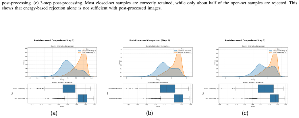
- Under post-processing, the pipeline still recovers roughly the right number of source groups even as cluster quality degrades, indicating that partial forensic structure survives heavy image transformation.
Where Pith is reading between the lines
- The paper does not specify where FSD features come from or how they are extracted; if the FSD extractor was trained or tuned on generator distributions that overlap the WILD open-set pool, the clustering result would largely reduce to re-clustering the FSD features, making the open-set discovery claim weaker than it appears.
- The same frozen-encoder-plus-forensic-trace fusion could plausibly extend beyond faces to other synthetic media such as video frames or audio, since the architecture does not depend on face-specific structure.
- A direct test of generalizability would be to apply Face-Trace to a generator released after the FSD model was built; if the discovery stage still forms coherent clusters, the representation is capturing transferable source traces rather than memorized training signals.
Editorial analysis
A structured set of objections, weighed in public.
Referee Report
Summary. Face-Trace proposes a three-stage pipeline for open-set synthetic face attribution: closed-set classification of known generators using a frozen I-JEPA encoder and a lightweight MLP head, energy-based rejection of unknown generators, and offline/incremental clustering of rejected samples using a fused representation of projected I-JEPA features and Forensic Self-Descriptions (FSD). The paper reports 96.73% closed-set accuracy, 71.25% balanced rejection accuracy, and clustering performance of ARI 0.81, NMI 0.90, and purity 87.74% on the WILD dataset, with additional experiments on post-processing robustness, multiple incremental splits, and cross-dataset streams. The central novelty claimed is non-transductive unknown-generator discovery without retraining the attribution or rejection modules.
Significance. If the results are accepted, the work would be a meaningful step beyond pure open-set rejection toward organizing unknown synthetic-face sources into coherent groups, and the incremental formulation has practical appeal. The paper is among the first to combine frozen I-JEPA embeddings with forensic descriptors for generator discovery, and it includes useful ablations (backbone, embedding type, clustering algorithm, HDBSCAN parameters, seed stability). The empirical basis is broad, with multiple generator splits and external datasets. However, the discovery-stage numbers are compromised by hyperparameter selection on the evaluation set, and the provenance of the FSD component is underspecified. These issues are substantial but addressable; with a clean evaluation protocol and full disclosure of the FSD model, the framework's contribution could be solid.
major comments (4)
- [§VIII-E (Table XV) and §VI-E] The HDBSCAN configuration (min_cluster_size=90, min_samples=15, epsilon=0.5) is selected on the WILD open-set pool by 'the best overall balance across ARI, NMI, purity, and number of discovered clusters'. This is selection on the same test data used to report the headline clustering results in Table IV; the 'number of discovered clusters' criterion also implicitly uses the known true U=10. Additionally, §VI-E states UMAP is fitted on the pool of energy-rejected samples before HDBSCAN. The reported ARI/NMI/purity therefore do not estimate performance on genuinely novel generators. A nested or split-protocol evaluation (e.g., tuning on one half of the open-set pool, reporting on the other) is required before the discovery claim can be trusted.
- [§IV-D and §VIII-D (Table XIV)] The FSD extractor is never specified: no model architecture, pretraining data, or training procedure is given, only that it 'produces a 960-dimensional descriptor of source-specific forensic microstructures derived from the image residuals'. Since the ablation shows FSD alone achieves ARI 0.66 while raw I-JEPA is 0.18 and CE-projected I-JEPA is 0.00, the discovery result rests largely on FSD. If the FSD extractor was trained or developed on the same generator distributions (including the WILD open-set generators), the fusion result would reduce to re-clustering FSD features. The paper must state the exact FSD model, its training set, and whether those data overlap with the evaluation generators.
- [Tables IV, V, and XIV] The reported clustering metrics are inconsistent across tables for what appears to be the same representation. Table IV gives Face-Trace ARI 0.81/NMI 0.90/purity 87.74%, Table V 'Plain' gives ARI 0.88/NMI 0.94/purity 89.20%, and Table XIV 'FSD + I-JEPA CE' gives identical values to Table V (0.88/0.94/89.20%). The captions suggest different subsets (energy-rejected vs. all open-set samples), but this is not stated in the main text, and Table IV is described only as 'organize rejected unknown samples'. The paper must clarify which subset each table uses, whether noise samples are excluded, and why the main discovery claim uses the lower numbers while the ablation reports higher ones on a superset.
- [§VI-F and §IX] The incremental promotion thresholds (buffer size 700, minimum support 300, cohesion 26, max buffering attempts 4) are selected by grid search on the 'initial reliable space' built from WILD open-set samples, maximizing purity while keeping the cluster count close to the true initialized generators. This is another use of test-set ground truth for hyperparameter selection. The 'in-the-wild' experiment (§VI-G) then reuses these thresholds, with only the minimum promotion size changed to 200. An independent validation split for the incremental parameters is needed to support the claim that the pipeline 'can operate in-the-wild'.
minor comments (5)
- [§IV-D] Please provide a citation or precise reference for the FSD extractor and its feature dimensionality. The current text refers to [31] but does not say whether the same pretrained model is used or if it is fine-tuned in this work.
- [§V-B and §VII-B] The default clustering metrics exclude noise-labelled samples (§V-B), but Table XV explicitly includes noise. This can change ARI/NMI/purity substantially; to avoid ambiguity, every table should state whether noise is included or excluded.
- [Appendix of author affiliations] The affiliation line contains a typo: 'Claudio SchiavellaStudent Member IEEE' should have a space (likely 'Claudio Schiavella, Student Member, IEEE').
- [General] No code, data splits, or trained models are released, so all numbers are currently non-reproducible. Sharing the embedding extraction scripts, FSD feature extraction code, and the exact WILD split would strengthen the paper substantially.
- [Table IV] The column header 'Kknown' should be 'K_known' or 'K known' for readability; as written it may be misread as a variable named Kknown.
Circularity Check
Unknown-generator discovery is partly fitted: HDBSCAN hyperparameters and the fused embedding are selected using ARI/NMI/purity and the expected cluster count on the same WILD open-set pool later reported as the discovery result.
specific steps
-
fitted input called prediction
[Section VIII-E (Table XV); Section VI-E; Section VII-B (Table IV)]
"increasing the parameters improves purity and leads to a number of clusters closer to the expected number of WILD open-set generators. The configuration with min cluster size = 90, min samples = 15, and ϵ = 0.5 achieves the best overall balance across ARI, NMI, purity, and number of discovered clusters. For this reason, it is adopted in the conducted experiments."
The final discovery settings are chosen by maximizing ARI/NMI/purity and cluster count on the same WILD open-set pool whose labels are used for the final Table IV scores. ARI/NMI require the true generator partition, and the 'expected number' is U=10, so Section III-C's claim that Q is not assumed known is not tested. The reported 10/10 cluster count and ARI 0.81/NMI 0.90/purity 87.74% are the outcome of test-set selection, not an independent prediction on novel generators.
-
fitted input called prediction
[Section VIII-D (Table XIV); Section VII-B (Table IV)]
"FSD features provide strong clustering performance, while the best results are obtained by fusing FSD with I-JEPA embeddings. In particular, the FSD + I-JEPA representation trained with CE achieves the highest average purity, showing that this combination produces the most discriminative space for unknown generator clustering."
The discovery representation is selected by ranking clustering metrics computed on the WILD open-set partition, and the same partition is later used to report the method's discovery metrics. The embedding choice is thus supervised by the true generator labels of the evaluation pool, making the headline clustering performance partly an artifact of the selection criterion rather than independent evidence that the representation discovers unseen generators.
full rationale
Face-Trace is primarily an empirical pipeline paper. Closed-set attribution is trained only on WILD closed-set generators; the energy threshold is calibrated on known samples at FPR 5%; and the FSD features are taken from separately published external work (ref. [31]), so these components are not circular. There is no load-bearing self-citation or imported uniqueness theorem; the WILD dataset has author overlap but is a public benchmark, and I-JEPA/DINOv3/CLIP/FSD are external. The circularity is confined to the discovery stage: HDBSCAN hyperparameters and the fused embedding are selected by evaluating ARI/NMI/purity (and implicitly the true number of unknown generators) on the very WILD open-set pool that is later reported as the discovery headline. This is selection on the test partition: the headline clustering metrics are partly fitted rather than predicted, and the paper's non-transductive 'Q not assumed known' claim is contradicted by using U=10 as a selection criterion. Because the exact ARI/NMI values still depend on the data and the closed-set/rejection results remain independent, this is partial circularity (6/10), not a definitional equivalence.
Axiom & Free-Parameter Ledger
free parameters (6)
- HDBSCAN parameters (offline) =
min_cluster_size=90, min_samples=15, epsilon=0.5
- UMAP parameters (offline) =
n_components=32, n_neighbors=15, min_dist=0.3
- Incremental buffer/promotion hyperparameters =
buffer_size=700, min_promotion=300, cohesion<26, max_attempts=4, HDBSCAN min_cluster_size=40/min_samples=5/epsilon=0.6
- Matching radius margin =
0.95 quantile + margin 0.95
- Energy temperature T =
1
- Rejection threshold tau =
FPR=5% on known samples
axioms (5)
- domain assumption Frozen pre-trained I-JEPA embeddings are a transferable representation for synthetic face attribution without any forensic-domain fine-tuning.
- domain assumption The FSD forensic descriptors from [31] adequately capture source-specific artifacts for unknown generator separation.
- domain assumption The WILD dataset generator partition (10 known / 10 unknown, 1000 images each) is representative of real open-set synthetic face attribution.
- standard math Mahalanobis distance with per-cluster covariance matrices is a valid similarity in the fused embedding space.
- domain assumption HDBSCAN can recover the unknown-generator structure from the UMAP-reduced fused representation.
Cite this review
Pith. "Pith review of Face-Trace: Open-Set Attribution and Progressive Discovery of Synthetic Face Generators." pith.science (2026). https://pith.science/paper/FLKO4DWI
@misc{pith2026260707545,
  author       = {Pith},
  title        = {Pith review of: Face-Trace: Open-Set Attribution and Progressive Discovery of Synthetic Face Generators},
  year         = {2026},
  howpublished = {\url{https://pith.science/paper/FLKO4DWI}},
  note         = {Machine review of arXiv:2607.07545}
}
read the original abstract
Recent advances in generative Artificial Intelligence have made synthetic face images increasingly realistic, creating new challenges for multimedia forensics. Source attribution methods should identify the generator of an image when the source is known, but also handle samples produced by unseen models. Most existing approaches, however, address synthetic face attribution in a closed-set setting, assuming that test samples can only originate from generators observed during training. This assumption does not hold in real-world scenarios, where new generators continuously appear and detecting an image as unknown is not sufficient, since rejected samples should also be organized according to their underlying sources. We introduce Face-Trace, a pipeline for open-set synthetic face source attribution that combines known generator classification, energy-based rejection, and unknown generator discovery. A classifier trained on frozen I-JEPA embeddings attributes known generators, while rejected samples are represented by combining projected I-JEPA features with complementary forensic traces and grouped to identify coherent sets of samples produced by unknown generators. We also extend the discovery stage to an incremental scenario, where rejected samples arrive over time. Experiments on the WILD dataset show 96.73% closed-set attribution accuracy, while rejection reaches 71.25% balanced accuracy and rejected samples are clustered into meaningful unknown-generator groups, with an Adjusted Rand Index of 0.81, a Normalized Mutual Information of 0.90, and an overall purity of 87.74%. In the incremental setting, the discovered generator space is progressively extended while maintaining a final purity of 99.23%, and cross-dataset experiments suggest that the pipeline can operate beyond the original data distribution.
Figures




Reference graph
Works this paper leans on
-
[1]
AI-synthesized faces are indistin- guishable from real faces and more trustworthy,
S. J. Nightingale and H. Farid, “AI-synthesized faces are indistin- guishable from real faces and more trustworthy,”Proc. Natl. Acad. Sci. U.S.A., vol. 119, no. 8, Art. no. e2120481119, Feb. 2022, doi: 10.1073/pnas.2120481119
-
[2]
Face deepfakes: A comprehensive review,
T. Fernando, D. Priyasad, S. Sridharan, A. Ross, and C. Fookes, “Face deepfakes: A comprehensive review,”arXiv preprint arXiv:2502.09812, 2025
Pith/arXiv arXiv 2025
-
[3]
Deepfake media forensics: State of the art and challenges ahead,
I. Amerini, M. Barni, S. Battiato, P. Bestagini, G. Boato, T. S. Bonaven- tura, V . Bruni, R. Caldelli, F. De Natale, R. De Nicola, L. Guarnera, S. Mandelli, G. L. Marcialis, M. Micheletto, A. Montibeller, G. Orr `u, A. Ortis, P. Perazzo, G. Puglisi, D. Salvi, S. Tubaro, C. M. Tonti, M. Villari, and D. Vitulano, “Deepfake media forensics: State of the art...
2025
-
[4]
Deepfake attribution: On the source identification of artificially generated images,
B. Khoo, R. C.-W. Phan, and C.-H. Lim, “Deepfake attribution: On the source identification of artificially generated images,”WIREs Data Mining Knowl. Discov., 2021, doi: 10.1002/widm.1438
-
[5]
Deepfake detection, attribution, and authentication: Insights from the FF4ALL project,
I. Amerini, M. Barni, S. Battiato, P. Bestagini, G. Boato, P. Bongini, V . Bruni, R. Casula, L. Cirillo, R. Caldelli, G. Daidone, F. De Natale, R. De Nicola, L. Guarnera, S. M. La Cava, S. Mandelli, G. L. Marcialis, M. Micheletto, A. Montibeller, V . Negroni, G. Orr`u, P. Perazzo, G. Puglisi, D. Salvi, B. Tondi, S. Tubaro, M. Villari, and D. Vitulano, “De...
2026
-
[6]
A unified survey on anomaly, novelty, open-set, and out-of- distribution detection: Solutions and future challenges,
M. Salehi, H. Mirzaei, D. Hendrycks, Y . Li, M. H. Rohban, and M. Sabokrou, “A unified survey on anomaly, novelty, open-set, and out-of- distribution detection: Solutions and future challenges,”Trans. Mach. Learn. Res., vol. 2022, 2022. PREPRINT. UNDER REVIEW. 13
2022
-
[7]
UMAP: Uniform manifold approximation and projection for dimension reduction,
L. McInnes, J. Healy, and J. Melville, “UMAP: Uniform manifold approximation and projection for dimension reduction,”arXiv preprint arXiv:1802.03426, 2020
Pith/arXiv arXiv 2020
-
[8]
Generalized out-of-distribution detection: A survey,
J. Yang, K. Zhou, Y . Li, and Z. Liu, “Generalized out-of-distribution detection: A survey,”Int. J. Comput. Vis., vol. 132, pp. 5635–5662, 2024, doi: 10.1007/s11263-024-02117-4
-
[9]
A baseline for detecting misclassified and out-of-distribution examples in neural networks,
D. Hendrycks and K. Gimpel, “A baseline for detecting misclassified and out-of-distribution examples in neural networks,” inProceedings of the 5th International Conference on Learning Representations (ICLR), 2017
2017
-
[10]
A benchmark for anomaly segmentation,
D. Hendrycks, S. Basart, M. Mazeika, M. Mostajabi, J. Steinhardt, and D. Song, “A benchmark for anomaly segmentation,”arXiv preprint arXiv:1911.11132, 2019
Pith/arXiv arXiv 1911
-
[11]
On the importance of gradients for detecting distributional shifts in the wild,
R. Huang, A. Geng, and Y . Li, “On the importance of gradients for detecting distributional shifts in the wild,” inAdvances in Neural Information Processing Systems (NeurIPS), 2021
2021
-
[12]
Energy-based out-of- distribution detection,
W. Liu, X. Wang, J. D. Owens, and Y . Li, “Energy-based out-of- distribution detection,” inAdvances in Neural Information Processing Systems, vol. 33, 2020, pp. 21464–21475
2020
-
[13]
GEN: Pushing the limits of softmax- based out-of-distribution detection,
X. Liu, Y . Lochman, and C. Zach, “GEN: Pushing the limits of softmax- based out-of-distribution detection,” inProc. IEEE/CVF Conf. Comput. Vis. Pattern Recognit. (CVPR), pp. 23946–23955, 2023
2023
-
[14]
Towards generalizable detector for generated image,
Q. Cai, C. Wu, Y . Zhang, J. Yu, and X. Tian, “Towards generalizable detector for generated image,”OpenReview, 2026. [Online]. Available: https://openreview.net/forum?id=MeawZGFIcT
2026
-
[15]
Deepfake network architecture attribution,
T. Yang, Z. Huang, J. Cao, L. Li, and X. Li, “Deepfake network architecture attribution,” inProc. AAAI Conf. Artif. Intell., vol. 36, no. 4, pp. 4662–4670, 2022, doi: 10.1609/aaai.v36i4.20391
-
[16]
RepMix: Representation mixing for robust attribution of synthesized images,
T. Bui, N. Yu, and J. Collomosse, “RepMix: Representation mixing for robust attribution of synthesized images,” inProceedings of the European Conference on Computer Vision (ECCV), 2022, pp. 146–163
2022
-
[17]
Progres- sive open space expansion for open-set model attribution,
T. Yang, D. Wang, F. Tang, X. Zhao, J. Cao, and S. Tang, “Progres- sive open space expansion for open-set model attribution,” inProc. IEEE/CVF Conf. Comput. Vis. Pattern Recognit. (CVPR), pp. 15856– 15865, 2023
2023
-
[18]
BOSC: A backdoor-based framework for open set synthetic image attribution,
J. Wang, B. Tondi, and M. Barni, “BOSC: A backdoor-based framework for open set synthetic image attribution,”IEEE Trans. Inf. Forensics Se- curity, vol. 20, pp. 8043–8058, 2025, doi: 10.1109/TIFS.2025.3592531
arXiv 2025
-
[19]
AdaParse: Personalized fingerprinting for visual generative model reverse engineering,
Y . Zheng, Z. Li, B. Yu, J. Zhou, and J. Lu, “AdaParse: Personalized fingerprinting for visual generative model reverse engineering,”IEEE Trans. Inf. Forensics Security, vol. 21, pp. 2682–2697, 2026, doi: 10.1109/TIFS.2026.3671095
arXiv 2026
-
[20]
S. Tang, P. He, H. Li, W. Wang, X. Jiang, and Y . Zhao, “Towards extensi- ble detection of AI-generated images via content-agnostic adapter-based category-aware incremental learning,”IEEE Trans. Inf. Forensics Secu- rity, vol. 20, pp. 2883–2898, 2025, doi: 10.1109/TIFS.2025.3546845
arXiv 2025
-
[21]
Beyond deepfake vs real: Facial deepfake detection in the open-set paradigm,
T. T. N. Bahavan, S. Seneviratne, S. Saha, K. Chen, S. Rasnayaka, and S. Halgamuge, “Beyond deepfake vs real: Facial deepfake detection in the open-set paradigm,”arXiv preprint arXiv:2503.08055, 2026
arXiv 2026
-
[22]
Learning transferable visual models from natural language supervi- sion,
A. Radford, J. W. Kim, C. Hallacy, A. Ramesh, G. Goh, S. Agarwal, G. Sastry, A. Askell, P. Mishkin, J. Clark, G. Krueger, and I. Sutskever, “Learning transferable visual models from natural language supervi- sion,” inProceedings of the 38th International Conference on Machine Learning (ICML), 2021, vol. 139, pp. 8748–8763
2021
-
[23]
O. Sim ´eoni, H. V . V o, M. Seitzer, F. Baldassarre, M. Oquab, C. Jose, V . Khalidov, M. Szafraniec, S. Yi, M. Ramamonjisoa, F. Massa, D. Haziza, L. Wehrstedt, J. Wang, T. Darcet, T. Moutakanni, L. Sentana, C. Roberts, A. Vedaldi, J. Tolan, J. Brandt, C. Couprie, J. Mairal, H. J ´egou, P. Labatut, and P. Bojanowski, “DINOv3,”arXiv preprint arXiv:2508.10104, 2025
Pith/arXiv arXiv 2025
-
[24]
Supervised contrastive learning for few-shot AI-generated image detection and attribution,
J. A. Urue ˜na, D. Camacho, and J. Huertas Tato, “Supervised contrastive learning for few-shot AI-generated image detection and attribution,” arXiv preprint arXiv:2511.16541, 2025
arXiv 2025
-
[25]
Generalizable synthetic image detection via language-guided contrastive learning,
H. Wu, J. Zhou, and S. Zhang, “Generalizable synthetic image detection via language-guided contrastive learning,”IEEE Trans. Artif. Intell., vol. 7, no. 6, pp. 3485–3496, 2026, doi: 10.1109/TAI.2025.3641104
arXiv 2026
-
[26]
DE-FAKE: Detection and attribution of fake images generated by text-to-image generation models,
Z. Sha, Z. Li, N. Yu, and Y . Zhang, “DE-FAKE: Detection and attribution of fake images generated by text-to-image generation models,” inProc. ACM SIGSAC Conf. Comput. Commun. Secur. (CCS), pp. 3418–3432, 2023, doi: 10.1145/3576915.3616588
arXiv 2023
-
[27]
Are CLIP features all you need for universal synthetic image origin attribution?,
D. Cioni, C. Tzelepis, L. Seidenari, and I. Patras, “Are CLIP features all you need for universal synthetic image origin attribution?,” inCom- puter Vision–ECCV 2024 Workshops, pp. 363–382, Cham, Switzerland: Springer, 2025, doi: 10.1007/978-3-031-92648-8 22
-
[28]
Zero-shot clustering of embeddings with pretrained and self-supervised learning encoders,
S. C. Lowe, J. B. Haurum, S. Oore, T. B. Moeslund, and G. W. Taylor, “Zero-shot clustering of embeddings with pretrained and self-supervised learning encoders,”OpenReview, 2024
2024
-
[29]
P. Sinhamahapatra, R. Koner, K. Roscher, and S. G ¨unnemann, “Is it all a cluster game? Exploring out-of-distribution detection based on clustering in the embedding space,”arXiv preprint arXiv:2203.08549, 2022
Pith/arXiv arXiv 2022
-
[30]
Towards discovery and attribution of open-world GAN generated images,
S. Girish, S. Suri, S. S. Rambhatla, and A. Shrivastava, “Towards discovery and attribution of open-world GAN generated images,” in Proc. IEEE/CVF Int. Conf. Comput. Vis. (ICCV), pp. 14094–14103, 2021
2021
-
[31]
T. D. Nguyen, A. Azizpour, and M. C. Stamm, “Forensic self- descriptions are all you need for zero-shot detection, open-set source attribution, and clustering of AI-generated images,”arXiv preprint arXiv:2503.21003, 2025
Pith/arXiv arXiv 2025
-
[32]
Autonomous and self- adapting system for synthetic media detection and attribution,
A. Azizpour, T. D. Nguyen, and M. C. Stamm, “Autonomous and self- adapting system for synthetic media detection and attribution,”arXiv preprint arXiv:2504.03615, 2025
Pith/arXiv arXiv 2025
-
[33]
Self-supervised learning from images with a joint-embedding predictive architecture,
M. Assran, Q. Duval, I. Misra, P. Bojanowski, P. Vincent, M. Rab- bat, Y . LeCun, and N. Ballas, “Self-supervised learning from images with a joint-embedding predictive architecture,” inProceedings of the IEEE/CVF Conference on Computer Vision and Pattern Recognition (CVPR), 2023, pp. 15619–15629
2023
-
[34]
Density-based clustering based on hierarchical density estimates,
R. J. G. B. Campello, D. Moulavi, and J. Sander, “Density-based clustering based on hierarchical density estimates,” inAdvances in Knowledge Discovery and Data Mining, J. Pei, V . S. Tseng, L. Cao, H. Motoda, and G. Xu, Eds. Berlin, Germany: Springer, 2013, vol. 7819, pp. 160–172, doi: 10.1007/978-3-642-37456-2 14
-
[35]
WILD: A new in-the-wild image linkage dataset for synthetic image attribution,
P. Bongini, S. Mandelli, A. Montibeller, M. Casu, O. Pontorno, C. Ragaglia, L. Zanchetta, M. Aquilina, T. Wani, L. Guarnera, B. Tondi, G. Boato, P. Bestagini, I. Amerini, F. G. B. De Natale, S. Battiato, and M. Barni, “WILD: A new in-the-wild image linkage dataset for synthetic image attribution,” inProc. Int. Joint Conf. Neural Netw. (IJCNN), 2025, pp. 1–8
2025
-
[36]
SFHQ-T2I: Synthetic faces from text-to-image models,
D. Beniaguev, “SFHQ-T2I: Synthetic faces from text-to-image models,” Kaggle, 2024, doi: 10.34740/KAGGLE/DSV/9548853
arXiv 2024
-
[37]
So-Fake: Benchmarking and explaining social media image forgery detection,
Z. Huang, T. Li, X. Li, H. Wen, Y . He, J. Zhang, H. Fei, X. Yang, X. Huang, B. Peng, and G. Cheng, “So-Fake: Benchmarking and explaining social media image forgery detection,”arXiv preprint arXiv:2505.18660, 2025
arXiv 2025
-
[38]
L. Lin, Santosh, M. Wu, X. Wang, and S. Hu, “AI-Face: A million- scale demographically annotated AI-generated face dataset and fairness benchmark,”arXiv preprint arXiv:2406.00783, 2025
Pith/arXiv arXiv 2025
-
[39]
Supervised contrastive learning,
P. Khosla, P. Teterwak, C. Wang, A. Sarna, Y . Tian, P. Isola, A. Maschinot, C. Liu, and D. Krishnan, “Supervised contrastive learning,” inAdvances in Neural Information Processing Systems, vol. 33, pp. 18661–18673, 2020
2020
-
[40]
Learning to discover novel visual categories via deep transfer clustering,
K. Han, A. Vedaldi, and A. Zisserman, “Learning to discover novel visual categories via deep transfer clustering,” inProceedings of the IEEE/CVF International Conference on Computer Vision (ICCV), 2019, pp. 8400–8408
2019
-
[41]
Generalized category discovery,
S. Vaze, K. Han, A. Vedaldi, and A. Zisserman, “Generalized category discovery,” inProceedings of the IEEE Conference on Computer Vision and Pattern Recognition (CVPR), 2022
2022
-
[42]
Parametric classification for generalized category discovery: A baseline study,
X. Wen, B. Zhao, and X. Qi, “Parametric classification for generalized category discovery: A baseline study,” inProceedings of the IEEE/CVF International Conference on Computer Vision (ICCV), 2023, pp. 16544– 16554
2023
-
[43]
ProtoGCD: Unified and unbiased prototype learning for generalized category discovery,
S. Ma, F. Zhu, X.-Y . Zhang, and C.-L. Liu, “ProtoGCD: Unified and unbiased prototype learning for generalized category discovery,”IEEE Trans. Pattern Anal. Mach. Intell., vol. 47, no. 7, pp. 6022–6038, 2025, doi: 10.1109/TPAMI.2025.3557502
arXiv 2025
-
[44]
Open-world deepfake attribution via confidence-aware asymmetric learning,
H. Zheng, N. Pu, W. Li, T. Long, N. Sebe, and Z. Zhong, “Open-world deepfake attribution via confidence-aware asymmetric learning,”arXiv preprint arXiv:2512.12667, 2025
arXiv 2025
-
[45]
On-the-fly category discovery,
R. Du, D. Chang, K. Liang, T. Hospedales, Y .-Z. Song, and Z. Ma, “On-the-fly category discovery,” inProc. IEEE/CVF Conf. Com- put. Vis. Pattern Recognit. (CVPR), pp. 11691–11700, 2023, doi: 10.1109/CVPR52729.2023.01125
arXiv 2023
-
[46]
Novel class discovery: An introduction and key concepts,
C. Troisemaine, V . Lemaire, S. Gosselin, A. Reiffers-Masson, J. Flocon- Cholet, and S. Vaton, “Novel class discovery: An introduction and key concepts,”arXiv preprint arXiv:2302.12028, 2023
Pith/arXiv arXiv 2023
-
[47]
On the generalised distance in statistics,
P. C. Mahalanobis, “On the generalised distance in statistics,”Sankhy ¯a A, vol. 80, no. 1, pp. 1–7, 2018, repr. fromProc. Nat. Inst. Sci. India, vol. 2, no. 1, pp. 49–55, 1936
2018
This paper was first reviewed by deepseek-v4-flash on August 2, 2026.
discussion (0)
Sign in with ORCID, Apple, or X to comment. Anyone can read and Pith papers without signing in.