REVIEW 4 major objections 5 minor 40 references
Projection-Based Correction for Enhancing Deep Inverse Networks
T0 review · 4 major / 5 minor · reviewed 2026-08-07 · deepseek-v4-flash
Pith's one-line read The paper claims that a fixed, non-iterative projection step applied after any trained deep inverse network enforces measurement consistency and improves reconstruction accuracy, and that it reduces to the identity for a well-trained…
desk verdict The noiseless projection is correct and gives real but modest gains; the noisy experiments are compromised by test-set leakage on λ, and the 'well-trained' theory is tautological. read the letter →
The pith
A machine-rendered reading of the paper's core claim, the machinery that carries it, and where it could break.
The reading
What carries the argument
The load-bearing object is the Euclidean projection onto the affine measurement-consistent set $\{x : Ax=y\}$, whose closed form is $\hat{x} = A^\dagger y + (I - A^\dagger A)\hat{f}(y)$, where $A^\dagger$ is the Moore-Penrose pseudoinverse. This operator replaces the inconsistent range-space component of the network output with the least-norm solution that satisfies $y=Ax$, while leaving the null-space component $(I - A^\dagger A)\hat{f}(y)$ untouched. For noisy measurements the machinery becomes the weighted projection $\hat{x} = (I + \lambda A^\top\Sigma^{-1}A)^{-1}(\hat{f}(y) + \lambda A^\top\Sigma^{-1}y)$, a one-step Tikhonov-type correction that can be precomputed for fixed $A,\Sigma$. The supporting theory is Definition 1 (well-trained network), Theorem 1 (the closed-form projection is the optimal solution of the constrained problem), and Theorem 2 (for well-trained networks the projection is the identity).
What would settle it
On a low-noise benchmark, compute the expected range-space error $\mathbb{E}\|A(\hat{f}(y)-x)\|^2$ and the expected null-space error $\mathbb{E}\|(I-A^\dagger A)(\hat{f}(y)-x)\|^2$ for a trained network: if the range-space error is not small relative to the null-space error, the projection cannot remove the dominant part of the error, and a test set where the projected output has lower PSNR than the raw network output would count directly against the paper's claim.
Extended reading notes
Core claim
The central claim is that the output of any trained deep inverse network can be written as a range-space component plus a null-space component, and that only the range-space component needs to be corrected for measurement consistency. The paper defines a well-trained network as one for which $\hat{f}(y) = A^\dagger y + (I - A^\dagger A)x$ holds over the data, and proves (Proposition 1) that such a network achieves zero mean-squared reconstruction error, and (Theorem 2) that the projection leaves its output unchanged. For a general network, the projection replaces the range-space part with $A^\dagger y$ and keeps the null-space part, so any inconsistency $A\hat{f}(y)\neq y$ is removed in one closed-form step. In the noisy case, the paper replaces the hard constraint by the penalty $(\hat{x} - \hat{f}(y))^\top(\hat{x}-\hat{f}(y)) + \lambda(A\hat{x}-y)^\top\Sigma^{-1}(A\hat{x}-y)$, with closed-form solution $\hat{x} = (I + \lambda A^\top\Sigma^{-1}A)^{-1}(\hat{f}(y) + \lambda A^\top\Sigma^{-1}y)$, and shows empirically that the optimal $\lambda$ decreases to zero as noise increases. Across deblurring, inpainting, and single-pixel imaging, the projection consistently improves PSNR/SSIM for convolutional, transformer, diffusion, and unrolled architectures, with the largest gains at low noise.
Load-bearing premise
The argument depends on the assumption that a trained network's reconstruction error lies almost entirely in the null space of the forward operator, so replacing the range-space component with the least-norm measurement-consistent value discards no meaningful signal information.
Editorial extensions
If this is right
- Any existing inverse network can be made exactly measurement-consistent in the noiseless case by one application of a fixed linear operator, with no retraining and no extra parameters.
- At low noise, the projection typically improves PSNR and SSIM, including on out-of-distribution test sets, acting as a generalization booster for data-driven solvers.
- For noisy measurements the method has a tunable knob: small $\lambda$ trusts the network, large $\lambda$ enforces the measurement, and the reported optimal values fall to zero as noise rises.
- Networks that already satisfy the range/null-space decomposition are untouched by the correction, so the method is a safe refinement rather than an alteration of a well-trained model.
- The magnitude of the gain tracks how much information the forward operator keeps: large gains appear in deblurring and inpainting, while single-pixel imaging at very low compression shows only small gains.
Reading between the lines
- A natural extension the paper does not develop is an adaptive noise-level rule for $\lambda$ (for instance, making it decrease with the noise variance), which the reported grid-search results suggest should work.
- Because the correction is a fixed linear map, it could be composed with other post-processing or generative refinement steps, or applied iteratively, without retraining; that may compound gains in settings with very strong priors.
- The method's behavior at high noise suggests that measurement consistency is not always desirable; a hybrid rule that switches the projection off when the estimated residual $A\hat{f}(y)-y$ is dominated by noise would address a limitation the paper explicitly flags.
- One could test the projector as a generic data-consistency layer inside untrained or equivariant imaging pipelines, since the projector needs no data to be constructed; this would connect it to broader unsupervised inverse-problem methods.
Editorial analysis
A structured set of objections, weighed in public.
Referee Report
Summary. The paper proposes a post-hoc projection step for deep inverse networks. For noiseless measurements y = Ax, the corrected estimate is x* = A†y + (I - A†A) f(y), the orthogonal projection of the network output onto the affine set {x : Ax = y}; the paper shows algebraically that this enforces measurement consistency and that for a 'well-trained' network the projection is the identity. For noisy measurements, a Tikhonov-style regularized variant (Eq. 17) with hyperparameter λ is proposed. Experiments on inpainting, deblurring, single-pixel imaging, and one spectral imaging problem compare network outputs before and after projection across several architectures and noise levels.
Significance. The noiseless projection is a correct and potentially useful drop-in consistency step: for y = Ax it is non-expansive with respect to the true x, so it cannot increase reconstruction error in the noiseless case, and Table 1 shows consistent, sometimes substantial gains (e.g., deblurring Unrolled PSNR 23.77 to 25.98). The paper is also commendable for releasing code and reporting a null-space consistency diagnostic (Eq. 18). However, the theoretical 'well-trained' analysis is tautological, the noisy-regime evaluation uses λ selected on the test set, and parts of the appendix appear to duplicate Table 1. Thus the broader claims of guaranteed improvement and rigorous theoretical support are not established in the current version, though the core noiseless idea is sound and fixable.
major comments (4)
- [§6.3, Table 2] The regularization parameter λ is chosen by a grid search against ground truth on the same test sets used for reporting ('we performed a grid search to select the optimal value for each noise level'; 'The best-performing λ was used to generate the final reconstruction results'). No validation split or repeated runs are described, so the noisy-regime results are affected by test-set leakage and lack error bars. In the σ = 0.10–0.30 rows the selected λ is 0 for several datasets, making Eq. (17) identical to the raw network output, and the remaining nonzero-λ rows show negligible or no improvement (e.g., σ = 0.20, Set3C PSNR 20.33 to 20.34; multiple SSIM values unchanged). Proposition 2 only computes the bias of a well-trained network and does not yield an optimal λ or an error expression for Eq. (17). The paper therefore does not establish the claimed improvement for noisy measurements.
- [Definition 1, Proposition 1, Theorem 2] A 'well-trained' network is defined by the conditions f(y) = A†y + N(y) and N(y) = (I - A†A)x for y = Ax, which immediately give f(y) = x. Consequently Proposition 1 (zero expected error) and Theorem 2 (projection reduces to identity) are true by construction. This is a tautology rather than a proof that trained networks satisfy the decomposition, and it does not explain the experimental behavior. The theoretical claim in the abstract ('we theoretically demonstrate...') should be reframed, or a nontrivial condition under which trained networks approximately satisfy Eqs. (4)–(5) should be provided.
- [Theorem 1, Appendix A] The proof of Theorem 1 multiplies by (AA^T)^-1 and uses A† = A^T(AA^T)^-1, which requires A to have full row rank. This assumption is missing from the theorem statement. For rank-deficient A, which is common in inverse problems, the proof is invalid. The closed-form formula (8) is nevertheless correct for the Moore-Penrose pseudoinverse when y ∈ R(A); please state the needed assumption or replace the proof with one based on the Moore-Penrose equations.
- [§6.2, Table 4] Several rows of Table 4 duplicate Table 1 exactly even though they are labeled for different datasets: Deblurring-Set3c and Inpainting-Set3c reproduce the DIV2K entries from Table 1. This indicates that the appendix does not actually contain the claimed evaluations on Set3c, CBSD68, and Urban100, so the cross-dataset generalization claim in Section 6.2 is unsupported. Moreover, some SPI SSIM values decrease after projection (e.g., Set3c DnCNN 0.544 to 0.540; Restormer 0.591 to 0.586), contradicting the blanket statement that the method improves all models. Please recompute these results and correct the tables.
minor comments (5)
- [§6.1] The text says 'four different datasets: DIV2K testing, Set3c, CBSD68, and Urban100, containing 3, 68, and 100 test images, respectively' but lists counts for only three datasets; please include the DIV2K test count.
- [Appendix A] The proof of Theorem 1 contains a typo: 'sing the constraint Ax = y' should be 'Using the constraint Ax = y'; also, Theorem 2's proof refers to 'SM, Appendix A' inconsistently with the actual appendix location.
- [Figure 1] The caption reads 'he measurement is processed' and should read 'The measurement is processed'.
- [Conclusion] The conclusion says the method was validated on 'PnP models', but the experiments in Section 6.2 use Unrolled, DnCNN, Restormer, and DiffUNet; no PnP model appears in Tables 1 or 4.
- [§5] When Σ is set to I, the meaning and scale of λ depend on the scaling of A and y; a sentence explaining the practical choice or range of λ would aid reproducibility.
Circularity Check
Well-trained identity theorems restate Definition 1, and noisy gains rely on test-set lambda selection; the noiseless projection itself is an independent, valid refinement.
-
self definitional
[Section 3, Definition 1 and Proposition 1 (proof in Appendix A)]
"The network ˆf is considered well-trained over a subset X0 ⊆ X if, for all x ∈ X0, ... (ii) The term N (y) accurately represents the component of x in the null space of A, such that N (y) = (I − A†A)x for all x ∈ X0. Proposition 1. ... Then, the expected reconstruction error over the training dataset satisfies E∥ ˆf (y) − x∥2 2 = 0."
Under the noiseless model y = Ax, condition (i) gives ˆf(y) = A†y + N(y) = A†Ax + N(y), and condition (ii) sets N(y) = (I − A†A)x. Substituting immediately yields ˆf(y) = x. Thus the zero-error conclusion of Proposition 1 is literally the definition of 'well-trained'; the Appendix proof only rewrites the definition. This makes the theorem true by construction, and it provides no evidence that any actually trained network satisfies the condition.
-
self definitional
[Section 4, Theorem 2]
"If the reconstruction network ˆf (y) is well-trained and contains a deep range-null-space decomposition, then the obtained solution using the projection-based correction is equivalent to the network output, i.e., the correction does not alter the final estimation."
Because Definition 1 already requires a well-trained network to output exactly x when y = Ax, any such output already lies in the feasible set {x : Ax = y}. The projection in Eq. (8) is the nearest point in that set to ˆf(y), so the identity is immediate. The proof in Appendix A only uses the null-space decomposition from Definition 1. The theorem is a restatement of the definition, not an independent result about trained deep networks.
1 more flagged steps
-
fitted input called prediction
[Section 6.3, Table 2]
"Since the projection introduces a regularization hyperparameter λ, we performed a grid search to select the optimal value for each noise level. ... The best-performing λ was used to generate the final reconstruction results, which are reported in Table 2."
The improvements attributed to the 'Projected' method in Table 2 are obtained after selecting λ by grid search against ground truth on the same test datasets (DIV2K Test, Set3C, CBSD68, Urban100) whose PSNR/SSIM are then reported. No held-out validation split or parameter-free selection rule is provided. In several high-noise rows the chosen λ is 0, making the projected result numerically identical to the network output, so the reported 'gains' are a consequence of test-set hyperparameter selection rather than an out-of-sample prediction.
full rationale
The paper contains two genuinely independent, non-circular components. The noiseless correction formula in Eq. (8) is derived from a constrained least-squares problem and is a standard orthogonal projection onto the affine set {x : Ax = y}; for any network output f(y), it satisfies Ax* = y and it strictly decreases (or preserves) the distance to the true x. That mathematical guarantee is self-contained and does not depend on the 'well-trained' definition. The empirical noiseless results in Table 1 are consistent with this projection property, so they are not 'forced by construction' in a harmful sense. The circularity lies in the theoretical framing: Definition 1 defines a well-trained network as one that already satisfies f(y) = x, and Proposition 1 and Theorem 2 then 'prove' consequences of that definition. These results are true by construction and give no independent evidence that real networks satisfy the condition; the paper's own null-space consistency metric (Eq. 18) shows the condition is only approximately met. The noisy-regime claim is further weakened because λ is chosen on the test data used for reporting, and several high-noise rows reduce to λ = 0, i.e., no correction. There is no load-bearing self-citation: Theorem 1 cites reference [16] and the decomposition is inspired by [28], but the proofs are included and do not depend on an unverified result from the same authors. Overall, the main projection operation has independent mathematical content, but the 'well-trained identity' theorems are definitional and the noisy improvement claim is partly fitted, so the paper receives a partial circularity score of 6 rather than 0 or 10.
Assumptions & free parameters
free parameters (1)
- lambda (regularization weight) =
grid-searched per dataset and noise level; examples include 0.001, 0.0005, 0.0001 in Table 2
assumptions (2)
- domain assumption A has full row rank so (AA^T)^-1 exists in the proof of Theorem 1
- ad hoc to paper The 'well-trained' condition in Definition 1 holds for real networks
Cite this review
Pith. "Pith review of Projection-Based Correction for Enhancing Deep Inverse Networks." pith.science (2026). https://pith.science/paper/GCOFV2WP
@misc{pith2026250515777,
  author       = {Pith},
  title        = {Pith review of: Projection-Based Correction for Enhancing Deep Inverse Networks},
  year         = {2026},
  howpublished = {\url{https://pith.science/paper/GCOFV2WP}},
  note         = {Machine review of arXiv:2505.15777}
}
read the original abstract
Deep learning-based models have demonstrated remarkable success in solving illposed inverse problems; however, many fail to strictly adhere to the physical constraints imposed by the measurement process. In this work, we introduce a projection-based correction method to enhance the inference of deep inverse networks by ensuring consistency with the forward model. Specifically, given an initial estimate from a learned reconstruction network, we apply a projection step that constrains the solution to lie within the valid solution space of the inverse problem. We theoretically demonstrate that if the recovery model is a well-trained deep inverse network, the solution can be decomposed into range-space and null-space components, where the projection-based correction reduces to an identity transformation. Extensive simulations and experiments validate the proposed method, demonstrating improved reconstruction accuracy across diverse inverse problems and deep network architectures.
Figures


Figures from the paper (2 more)


Reference graph
Works this paper leans on
-
[16]
Liang J, Cao J, Sun G, Zhang K, Van Gool L and Timofte R 2021 Swinir: Image restoration using swin transformer Proceedings of the IEEE/CVF international conference on computer visionpp 1833–1844
work page 2021
-
[1]
Projection-Based Correction for Enhancing Deep Inverse Networks
Introduction Linear inverse problems are fundamental in computational imaging, signal processing, and various scientific and engineering applications [1, 2]. Mathematically, an inverse problem involves recovering an unknown signal x ∈ Rn from indirect or incomplete measurements y ∈ Rm, modeled as: y = Ax + n, (1) where A ∈ Rm×n represents the linear forwa...
work page Pith review arXiv 2025
-
[2]
Related W ork Deep inverse models have gained significant attention for solving ill-posed inverse problems by leveraging data-driven approaches to approximate the inverse mapping of complex measurement processes, surpassing traditional iterative optimization algorithms. Data-Driven Inverse Models. Supervised deep learning approaches aim to learn an advanc...
-
[3]
Deep Inverse Networks A common approach to solving inverse problems is to leverage supervised learning techniques. Given a training dataset consisting of paired observations ( x, y), a reconstruction network f is trained by minimizing the following objective function ˆf ∈ arg min f Ex,y∥f (y) − x∥2 2, (3) where the optimal estimator is the minimum mean sq...
-
[4]
Consequently, the learned function ˆf (y) is influenced by the structure and diversity ofXo, which means that the model may fail to generalize well to out-of-distribution samples. To formalize the conditions under which a reconstruction network can be considered well-trained, we introduce the following theoretical framework, which will be further explored...
-
[5]
Projection-Based Correction Despite the optimization process described in Eq. 3, the estimated reconstruction ˆf (y) may not fully conform to the measurement model due to limitations in the training procedure. In particular, it is often the case that A ˆf (y) ̸= y, which implies that the residual error, ∥A ˆf (y) − y∥2 2 is nonzero. This discrepancy arise...
-
[6]
Regularized Projection-Based Correction for Noisy Measurements When noise is present in the measurement model, the standard projection-based correction method no longer guarantees optimal reconstruction. Specifically, the following proposition shows that a well-trained network exhibits a bias influenced by the covariance of the noise. Proposition 2. Let ˆ...
-
[7]
We conducted three main experiments to assess its impact
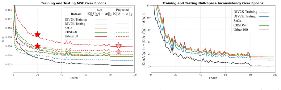
Simulations and Results In this section, we evaluate the effectiveness of our proposed Projection-Based Correction approach in enhancing deep inverse networks under both noiseless and noisy conditions. We conducted three main experiments to assess its impact. The first experiment examines the role of the Projection-Based Correction step during training by...
Show all 40 references
-
[8]
Visual results of the evaluated method
(18) Figure 3. Visual results of the evaluated method. The leftmost column shows the measurement and the ground truth (GT). The results at an early epoch (20 epochs) and the final epoch (100 epochs) are displayed to assess the effect of the Projection-Based Correction method. ...
-
[9]
Conclusion This work introduced a Projection-Based Correction method to enhance deep inverse networks by enforcing strict measurement consistency, addressing a key limitation of deep learning-based solvers that often violate physical constraints. Through extensive evaluations ...
-
[10]
Thus, we obtain E∥x − ˆf (y)∥2 2 = Tr(A†Σ(A†)⊤)
(44) From standard properties of Gaussian noise: E∥A†n∥2 2 = Tr(A†Σ(A†)⊤), (45) where Σ is covariance matrix of the noise. Thus, we obtain E∥x − ˆf (y)∥2 2 = Tr(A†Σ(A†)⊤). (46) Appendix B This section shows additional results for different testing datasets of experiment 6.2 of...
-
[11]
Ongie G, Jalal A, Metzler C A, Baraniuk R G, Dimakis A G and Willett R 2020 IEEE Journal on Selected Areas in Information Theory1 39–56
2020
-
[12]
Bacca J, Martinez E and Arguello H 2023 JOSA A 40 C115–C125
2023
-
[13]
Ronneberger O, Fischer P and Brox T 2015 U-net: Convolutional networks for biomedical image segmentation Medical image computing and computer-assisted intervention–MICCAI 2015: 18th international conference, Munich, Germany, October 5-9, 2015, proceedings, part III 18(Springer...
2015
-
[14]
Zhang K, Zuo W, Chen Y, Meng D and Zhang L 2017 IEEE transactions on image processing26 3142–3155
2017
-
[15]
Zhang K, Li Y, Zuo W, Zhang L, Van Gool L and Timofte R 2021 IEEE Transactions on Pattern Analysis and Machine Intelligence44 6360–6376
2021
-
[17]
Zamir S W, Arora A, Khan S, Hayat M, Khan F S and Yang M H 2022 Restormer: Efficient transformer for high-resolution image restoration Proceedings of the IEEE/CVF conference on computer vision and pattern recognitionpp 5728–5739
2022
-
[18]
Choi J, Kim S, Jeong Y, Gwon Y and Yoon S 2021 arXiv preprint arXiv:2108.02938
2021 arXiv
-
[19]
Chan S H, Wang X and Elgendy O A 2016 IEEE Transactions on Computational Imaging3 84–98
2016
-
[20]
Romano Y, Elad M and Milanfar P 2017 SIAM Journal on Imaging Sciences10 1804–1844
2017
-
[21]
Monga V, Li Y and Eldar Y C 2021 IEEE Signal Processing Magazine38 18–44
2021
-
[22]
Arridge S, Maass P, ¨Oktem O and Sch¨ onlieb C B 2019Acta Numerica 28 1–174
-
[23]
Adler J and ¨Oktem O 2018 IEEE transactions on medical imaging37 1322–1332
2018
-
[24]
Shah V and Hegde C 2018 Solving linear inverse problems using gan priors: An algorithm with provable guarantees 2018 IEEE international conference on acoustics, speech and signal processing (ICASSP) (IEEE) pp 4609–4613
2018
-
[25]
Chen D and Davies M E 2020 Deep decomposition learning for inverse imaging problems Computer Vision– ECCV 2020: 16th European Conference, Glasgow, UK, August 23–28, 2020, Proceedings, Part XXVIII 16 (Springer) pp 510–526
2020
-
[26]
Sønderby C K, Caballero J, Theis L, Shi W and Husz´ ar F 2016 arXiv preprint arXiv:1610.04490
2016 arXiv
-
[27]
Schwab J, Antholzer S and Haltmeier M 2019 Inverse Problems 35 025008
2019
-
[28]
G¨ oppel S, Frikel J and Haltmeier M 2023 arXiv preprint arXiv:2309.06573
2023 arXiv
-
[29]
Angermann C, G¨ oppel S and Haltmeier M 2023 arXiv preprint arXiv:2304.06955
2023 arXiv
-
[30]
Wang Y, Yu J and Zhang J 2022 arXiv preprint arXiv:2212.00490
2022 arXiv
-
[31]
Hanke M 1997 Inverse problems 13 79
1997
-
[32]
Gupta H, Jin K H, Nguyen H Q, McCann M T and Unser M 2018 IEEE transactions on medical imaging 37 1440–1453
2018
-
[33]
Raj A, Li Y and Bresler Y 2019 Gan-based projector for faster recovery with convergence guarantees in linear inverse problems Proceedings of the IEEE/CVF international conference on computer visionpp 5602–5611
2019
-
[34]
Rick Chang J, Li C L, Poczos B, Vijaya Kumar B and Sankaranarayanan A C 2017 One network to solve them all–solving linear inverse problems using deep projection models Proceedings of the IEEE International Conference on Computer Visionpp 5888–5897
2017
-
[35]
Mardani M, Sun Q, Donoho D, Papyan V, Monajemi H, Vasanawala S and Pauly J 2018 Advances in Neural Information Processing Systems31
2018
-
[36]
Daras G, Chung H, Lai C H, Mitsufuji Y, Ye J C, Milanfar P, Dimakis A G and Delbracio M 2024 arXiv preprint arXiv:2410.00083
2024 arXiv
-
[37]
Tachella J, Chen D, Hurault S, Terris M and Wang A 2023 DeepInverse: A deep learning framework for inverse problems in imaging URL https://github.com/deepinv/deepinv
2023
-
[38]
Chen D, Tachella J and Davies M E 2021 Equivariant imaging: Learning beyond the range space Proceedings of the IEEE/CVF International Conference on Computer Visionpp 4379–4388
2021
-
[39]
Huang T, Dong W, Yuan X, Wu J and Shi G 2021 Deep gaussian scale mixture prior for spectral compressive imaging Proceedings of the IEEE/CVF Conference on Computer Vision and Pattern Recognitionpp 16216– 16225
2021
-
[40]
Wang J, Zhang Y, Yuan X, Meng Z and Tao Z 2022 Modeling mask uncertainty in hyperspectral image reconstruction European Conference on Computer Vision(Springer) pp 112–129
2022
Reviewed August 7, 2026 · model on record in the stance chip above.
Discussion (0). Continue with ORCID to comment.