REVIEW 3 major objections 8 minor 22 references
No stable subspace to track: GaLore's gradient space is noise
Reviewed by Pith at T0; open to challenge. T0 means a machine referee read the full paper against a public rubric. the ladder, T0–T4 →
T0 review · glm-5.2
2026-07-08 21:48 UTC pith:GTD5WN2P
load-bearing objection Solid paper with a genuinely new measurement at its core; the theoretical extension rests on an untested assumption but the empirical findings stand on their own. the 3 major comments →
No Subspace to Track: Non-Identifiability and Optimizer State in Low-Rank Training
The pith
A machine-rendered reading of the paper's core claim, the machinery that carries it, and where it could break.
Core claim
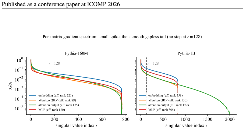
The central object is the reproducible rank k*, the number of gradient directions that two same-step split-batch estimates of the top-r subspace share. At Pythia-160M with r=128, k* is approximately 39, and it shrinks with scale (from about 50 at 70M to about 21 at 6.9B). The paper establishes that k* is the measurable boundary between a genuine low-rank structure in the gradient (the small dominant spike documented in prior work) and a gapless spectral tail whose directions are statistically non-identifiable: they are redrawn with each sample, not tracked over time. The non-identifiability is a property of the gradient itself, not of GaLore, since every model measured was trained with full-
What carries the argument
chordal (principal-angle) Frobenius distance between orthonormal frames; Davis-Kahan perturbation theory for near-degenerate singular directions; Haar-random model for redrawn directions; Weingarten calculus on the orthogonal group for the blind-estimator lower bound; power-law spectral tail with exponent 1.03-1.35; forgetting-factor bias-variance tradeoff for beta2 prescription
Load-bearing premise
The Haar-random model for the redrawn directions assumes the non-reproducible directions are uniformly randomly oriented within the degenerate spectral block, which is the standard limiting case when the spectral gap vanishes. The actual gradient covariance tail has a power-law spectrum rather than a flat one, so if the tail eigenvalues have structured anisotropy that persists across samples, the suboptimality bound and the optimal transport rule could differ from the isotrop
What would settle it
If two same-step split-batch estimates of the top-r gradient subspace were found to agree substantially more than two estimates taken T steps apart, the non-identifiability claim would fail: the rotation would carry genuine information about elapsed time rather than being dominated by estimator noise.
If this is right
- Before trusting any rank-r gradient projection, practitioners should split a batch, compute the subspace twice, and count the agreeing directions (k*). If r exceeds k*, the excess directions are noise being refreshed, and the optimizer state should be transported through the rotation rather than carried blindly.
- The SVD computation that GaLore performs at each refresh is largely wasted beyond the first k* directions: a random projection that includes the spike directions would capture comparable gradient energy, suggesting cheaper alternatives are viable, especially late in training when k* is smallest.
- The finding that non-identifiability strengthens with scale (k* shrinks from 50 at 70M to 21 at 6.9B) implies that the gap between nominal rank and reproducible rank widens for larger models, making state transport and shorter second-moment memory increasingly important at scale.
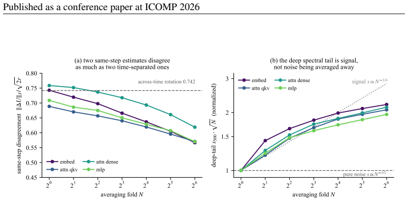
- The N^(-1/4) scaling of the spectral tail under averaging means that any method attempting to stabilize the subspace by accumulating gradient samples faces a fundamental signal, not a noise, barrier, and no practical averaging window will open a spectral gap at r.
Editorial analysis
A structured set of objections, weighed in public.
Referee Report
Summary. This paper investigates whether the top-r gradient subspace that GaLore-family optimizers recompute every T steps is a well-defined, trackable object. Using a same-step split-batch control, the authors show that two estimates of the subspace computed at the same step from disjoint minibatches disagree by 0.725√(2r), essentially the same as the 0.742√(2r) rotation measured across a full refresh interval. This implies the apparent per-refresh rotation is dominated by estimator noise rather than motion of a stable subspace. Only k*≈39 of r=128 directions are reproducible. The authors trace this to a gapless gradient spectrum at rank r, show that averaging cannot resolve it (the tail shrinks as N^{-1/4} rather than N^{-1/2}), and demonstrate the effect across four model families, three architecture classes, and scales from 70M to 6.9B. They then show that basis averaging fails to help, while transporting optimizer state through the rotation (the LDAdam rule) and shortening the second-moment memory (β2=0.99) both improve perplexity, with a full-rank control reversing the β2 preference.
Significance. The central non-identifiability measurement is well-designed and the same-step control is a clean experimental design that cleanly separates estimator noise from genuine drift. The cross-backend replication (0.3% difference between NVIDIA and AMD) and the trajectory control (five checkpoints along training) rule out numerical artifacts and the pretrained-checkpoint objection respectively. The k* count is a direct measurement with no fitted parameters, and the Weingarten lower bound (Theorem 1) is a parameter-free derivation. The N^{-1/4} averaging scaling is a falsifiable empirical claim confirmed across scales. The 2×2 controlled experiment at 1B (Table 1) with three seeds per cell and the full-rank causal control (Figure 5) are well-constructed. The paper provides a clear, actionable prescription (measure k*; transport state; lower β2) grounded in the measurement. The main theoretical contribution—the Weingarten bound and the MMSE transport rule—depends on a Haar-isotropy assumption whose sensitivity is not directly tested, which is the primary concern detailed below.
major comments (3)
- Appendix B, Theorem 1 and Remark 2: The Weingarten lower bound of (r−k*)/2 ≈ 45× suboptimality for blind second-moment carry depends on R ~ Haar(O(r−k*)), the fully-degenerate limit. The paper justifies this via Davis–Kahan (§3.3): as the spectral gap vanishes, perturbation sensitivity is maximal, so sub-threshold directions redraw freely. However, Davis–Kahan bounds the magnitude of perturbation sensitivity; it does not guarantee that the perturbation is isotropic (Haar-uniform). The gradient covariance tail has a power-law spectrum (α=1.03–1.35, §3.5), not a flat one. If the tail eigenvectors carry persistent anisotropic structure across samples, the redrawn directions would be biased rather than Haar-uniform, making the (r−k*)/2 bound an overestimate and potentially changing the optimal transport rule from the isotropic R² map of Proposition 3. The paper acknowledges this in AppendixC
- The indirect validation of Haar-isotropy is that the same-step disagreement of 0.725√(2r) sits below the Haar ceiling of √(2r). But this is a weak test: any distribution with non-trivial correlations between consecutive draws would also produce a value below √(2r). A direct test would compare the full distribution of rotation matrix entries (e.g., the empirical distribution of singular values of R = U_new^T U_old, or the distribution of individual R_{ij}² entries) against the Haar predictions of Eq. (6) (Beta(1/2, (r-1)/2) marginals, specific fourth-moment relations). Without such a test, the (r−k*)/2 suboptimality factor and the optimality of the isotropic transport rule are conditional on an unverified assumption. This is load-bearing because the bound quantifies the cost of blind carry and motivates the transport prescription.
- Table 1: The transport arm is the full LDAdam update, which combines state transport with error feedback. The paper acknowledges this (§5.2, 'this experiment does not separate the contribution of transport from that of error feedback'). However, the optimality statements (Proposition 3, Theorem 1) concern only the transport rule, while the empirical advantage of 18.73 vs 19.28 may be substantially or entirely due to error feedback. This confounds the theoretical contribution with an orthogonal engineering technique. An ablation isolating transport (R applied to moments, no error feedback) from error feedback alone would be needed to support the claim that transport is the mechanism driving the improvement.
minor comments (8)
- §3.2: The statement 'only k*≈39 of the r=128 directions the top-r cut returns are reproducible across the split' should specify the threshold used to classify a direction as 'reproducible.' Is this based on a principal-angle threshold, a singular-value threshold of the cross-Gram matrix, or something else? The protocol in Appendix F defines k*(N) = r·ov where ov = Σ σ_i(U_1^T U_2)²/r, which is a continuous quantity; the discrete count of 39 appears to involve an implicit threshold.
- Figure 3a: The y-axis label 'same-step disagreement ||ΔU||_F / √(2r)' and the dashed line at 0.742 are clear, but it would help to also mark the Haar ceiling (1.0) explicitly on the plot for reference.
- §5.3: The canonical-GaLore β2 margin is described as 'hardware-sensitive' with a matched-recipe run on a different GPU backend not reproducing it. This is concerning for reproducibility. It would strengthen the paper to state which backend produced which result and whether the SVD implementation (e.g., different LAPACK routines) could explain the discrepancy.
- Table 3 (Appendix E): The APOLLO-Mini row reports two values per β2 cell (99.8/101.77 and 96.76/97.20) without explanation. These appear to be two seeds, but this should be stated explicitly, and the mean±std format used for other rows should be applied for consistency.
- §4: The claim that GaLore retains 'a roughly constant γ_g ≈ 0.67–0.73 of the squared gradient throughout, regardless of the redraw' is important for the energy-capture argument. It would help to show this quantity over training (a figure or table) rather than stating it inline, since it is a key part of the reconciliation argument.
- Appendix C, Proposition 3: The isotropy assumption is stated as 'exact only in the near-degenerate tail.' The proof assumes g ~ N(0, σ²I), which is a stronger assumption than second-order isotropy. The text should clarify whether the result requires full Gaussian isotropy or only second-moment isotropy, since the gradient distribution is likely non-Gaussian.
- The paper uses 'k⋆' (with a star) in some places and 'k*' (with an asterisk) in others. Standardize notation throughout.
- §3.6: The ViT-B result (0.53 of maximal) is described as 'more weakly' present. It would be useful to briefly discuss why the effect is weaker in vision—whether this is due to a smaller gradient dimension, different spectral properties, or the CIFAR-10 dataset.
Simulated Author's Rebuttal
We thank the referee for a careful and substantive review. The three major comments are interconnected: they concern (1) whether the Haar-isotropy assumption underlying Theorem 1 is directly tested, (2) whether the indirect validation (same-step disagreement below the Haar ceiling) is sufficient, and (3) whether the Table 1 transport experiment isolates transport from error feedback. We agree that the Haar assumption is load-bearing and insufficiently tested, and we will add a direct distributional test. We also agree that the transport/error-feedback confound is a real limitation and will add an ablation. We push back on one point: the referee's concern that anisotropic tail structure would change the qualitative conclusion, which we address on the merits.
read point-by-point responses
-
Referee: The Weingarten lower bound of (r-k*)/2 suboptimality depends on R ~ Haar(O(r-k*)), the fully-degenerate limit. Davis-Kahan bounds perturbation sensitivity magnitude but does not guarantee isotropic (Haar-uniform) perturbation. The gradient covariance tail has a power-law spectrum (alpha=1.03-1.35), not a flat one. If tail eigenvectors carry persistent anisotropic structure, the bound could be an overestimate and the optimal transport rule could change from the isotropic R^2 map of Proposition 3.
Authors: The referee is correct that Davis-Kahan establishes maximal perturbation sensitivity but does not, by itself, guarantee Haar-uniformity of the redrawn directions. The gap between 'maximally sensitive' and 'isotropically distributed' is real, and the manuscript currently bridges it by assertion rather than by direct test. We accept this criticism. In the revision we will add a direct distributional test of the Haar hypothesis on the (r-k*) non-reproducible directions, as detailed in our response to the second comment below. We note one point on the merits: the power-law spectrum (alpha=1.03-1.35) characterizes the singular-value distribution within the tail, not necessarily the eigenvector distribution. A power-law in singular values is compatible with Haar-uniform eigenvectors (as in spiked covariance models with a bulk). The referee's concern is about persistent anisotropic structure in the eigenvectors specifically, which is the right question and is testable. If the test reveals anisotropy, the (r-k*)/2 bound would indeed be an overestimate of the blind-carry cost, though the qualitative conclusion (blind carry is suboptimal; transport helps) would survive as long as any non-trivial rotation occurs. We will state this conditional structure explicitly in the revised Theorem 1 and Remark 2. revision: yes
-
Referee: The indirect validation of Haar-isotropy (same-step disagreement of 0.725*sqrt(2r) below the Haar ceiling of sqrt(2r)) is a weak test: any distribution with non-trivial correlations between consecutive draws would also produce a value below sqrt(2r). A direct test would compare the full distribution of rotation matrix entries (e.g., empirical distribution of singular values of R = U_new^T U_old, or distribution of individual R_{ij}^2 entries) against Haar predictions of Eq. (6) (Beta(1/2, (r-1)/2) marginals, specific fourth-moment relations). Without such a test, the (r-k*)/2 suboptimality factor and the optimality of the isotropic transport rule are conditional on an unverified assumption.
Authors: We agree completely. The same-step disagreement sitting below the Haar ceiling is a necessary but not sufficient condition, and we should not have presented it as validation of Haar-isotropy. We will add the direct test the referee proposes. Specifically, using the existing split-batch protocol (Appendix F), we will extract the rotation matrix R restricted to the non-reproducible (r-k*) directions and test: (i) the marginal distribution of R_{ij}^2 entries against the Beta(1/2, (r-1)/2) prediction of Eq. (6); (ii) the fourth-moment relations E[R_{ij}^4] = 3/(r(r+2)) and E[R_{ij}^2 R_{ik}^2] = 1/(r(r+2)) for j != k; and (iii) the singular-value distribution of R against the Marchenko-Pastur-type prediction for Haar-distributed subblocks. This test uses data we already collect (the cross-Gram matrix U_1^T U_2 from the split-batch probe) and requires no new experiments, only new analysis. We will report the results whatever they show. If the Haar hypothesis is rejected, we will re-derive the bound under the empirically measured anisotropy and adjust the suboptimality factor and transport rule accordingly. The first-moment transport rule (Proposition 3) is exact under any rotation R, not just Haar R, so it is unaffected; only the second-moment blind-carry bound (Theorem 1) and the optimality of the isotropic R^2 map for the second moment depend on Haar. revision: yes
-
Referee: Table 1: The transport arm is the full LDAdam update, combining state transport with error feedback. The optimality statements (Proposition 3, Theorem 1) concern only the transport rule, while the empirical advantage of 18.73 vs 19.28 may be substantially or entirely due to error feedback. This confounds the theoretical contribution with an orthogonal engineering technique. An ablation isolating transport (R applied to moments, no error feedback) from error feedback alone would be needed to support the claim that transport is the mechanism driving the improvement.
Authors: This is a fair and important criticism. The manuscript already acknowledges the confound (Section 5.2: 'this experiment does not separate the contribution of transport from that of error feedback'), but acknowledging a confound is not the same as resolving it, and the referee is right that the current Table 1 cannot support the claim that transport is the mechanism. We will add the ablation the referee requests: a 2x2 factorial crossing {transport, no transport} x {error feedback, no error feedback} at the same 1B/40K recipe, with at least three seeds per cell. This isolates the transport contribution from error feedback. We note that the theoretical contribution (Proposition 3 and Theorem 1) does not depend on this experiment: Proposition 3 proves first-moment transport is the MMSE linear map under isotropic gradients, and Theorem 1 proves blind second-moment carry is (r-k*)/2 suboptimal, both as mathematical results. What the ablation tests is whether the theoretical advantage of transport translates to empirical perplexity gains independent of error feedback. If transport alone (without error feedback) does not improve over carry, we will say so plainly and re-scope the empirical claim accordingly. We will also soften the language in Section 5.2 to make clear that the current Table 1 supports only the joint effect of transport plus error feedback, not transport in isolation, pending the ablation results. revision: yes
Circularity Check
No significant circularity: the central non-identifiability claim is measured directly against external benchmarks with no fitted parameters, and theoretical results are parameter-free derivations from stated assumptions.
full rationale
The paper's central claim — that the top-r gradient subspace is statistically non-identifiable beyond a small reproducible core — is established by a direct measurement (same-step split-batch disagreement ≈ across-time rotation, 0.73√(2r) vs 0.74√(2r)) with no fitted parameters. The reproducible rank k*≈39 is a direct count from the same split-batch protocol, not a prediction from a fitted model. The Weingarten lower bound (Theorem 1, Appendix B) is a parameter-free derivation from Haar-randomness assumptions: it uses standard second- and fourth-order moments of Haar-distributed entries (Eq. 6-7) to compute the suboptimality factor (r+4)/2 for blind carry, with no input that encodes the output. Proposition 3 (first-moment transport as MMSE) is a standard linear estimation result under isotropy. Proposition 4 (coverage equals cumulative spectral mass) is a trace identity. The paper explicitly flags where two estimators read from the same data (§3.4: 'Both readings derive from the same measurement, so this is a consistency check between two estimators rather than an independent prediction'), which is transparent rather than circular. The Haar-isotropy assumption is a modeling assumption whose sensitivity is a correctness concern (noted by the reader and acknowledged in Appendix C), not a circularity: the bound's output (suboptimality factor) is not defined in terms of its input (the λ vector), and the assumption is externally falsifiable. No self-citation chain is load-bearing: the paper cites Davis-Kahan, Weingarten calculus, and Gur-Ari et al. as independent results, and the LDAdam transport rule (Robert et al., 2025) is treated as a known method whose optimality the paper independently characterizes. The derivation chain is self-contained.
Axiom & Free-Parameter Ledger
free parameters (4)
- k* (reproducible rank) =
~39 at Pythia-160M, r=128
- beta2 for shorter memory =
0.99
- beta3 (EMA-basis decay) =
{0, 0.9, 0.99, 0.999, 0.9999}
- noise scale nu_1 per layer (BBP model) =
calibrated to N=1 overlap
axioms (4)
- standard math Davis-Kahan / Wedin sin-theta theorem: subspace rotation is bounded by perturbation size over the spectral gap.
- domain assumption Haar-randomness of redrawn directions: the r-k* non-reproducible directions are uniformly distributed on the orthogonal group O(r-k*).
- domain assumption Gradient isotropy in the tail: the gradient covariance in the degenerate block is proportional to identity.
- domain assumption The gradient spectral tail follows a power law with exponent alpha=1.03-1.35.
read the original abstract
Memory-efficient optimizers such as GaLore train large language models by projecting gradients onto a rank-r subspace recomputed every T steps, assuming this subspace is a slowly drifting object that can be tracked. We show that beyond a small reproducible core, there is no such object. Two estimates of the top-r subspace computed at the same step from disjoint minibatches disagree as much as estimates computed T steps apart (0.73 vs 0.74 of the maximal chordal distance sqrt(2r), at Pythia-160M with r=128): the apparent rotation at each refresh is dominated by estimator noise. This holds across four model families in three architecture classes from 70M to 6.9B parameters, strengthening with scale, and more weakly in a vision transformer. Only ~39 of 128 directions are reproducible across minibatches, and averaging cannot recover the rest: under N-fold averaging the gradient's spectral tail shrinks as N^(-1/4) rather than the N^(-1/2) of pure noise, so no averaging budget makes the subspace well defined. What helps instead follows from treating each refresh as a change of coordinates for Adam's state. Carrying the second moment blindly is provably about (r-k*)/2 worse than the best rotation-blind estimator, while the first moment transports exactly through the rotation, the optimal linear map under isotropic gradients and the rule LDAdam uses. At 1B over 40k steps (3 seeds), full LDAdam reaches 18.7 perplexity at beta2=0.999, beating untransported GaLore after its best beta2 fix (19.3); shortening the second-moment memory to beta2=0.99 helps the refreshing optimizers, though for canonical GaLore the effect is small and a full-rank control reverses it. One measurable fact, subspace non-identifiability, clarifies why GaLore works, which patches work, and what to check before trusting a low-rank assumption: the reproducible rank k*.
Figures



Reference graph
Works this paper leans on
-
[1]
Online Identification and Tracking of Subspaces from Highly Incomplete Information
arXiv:1006.4046. Thomas Bendokat, Ralf Zimmermann, and P.-A. Absil. A Grassmann manifold handbook: Ba- sic geometry and computational aspects.Advances in Computational Mathematics,
work page internal anchor Pith review Pith/arXiv arXiv
-
[2]
A Grassmann Manifold Handbook: Basic Geometry and Computational Aspects
arXiv:2011.13699. Stella Biderman, Hailey Schoelkopf, Quentin Anthony, Herbie Bradley, et al. Pythia: A suite for analyzing large language models across training and scaling. InICML,
work page internal anchor Pith review Pith/arXiv arXiv 2011
-
[3]
13 Published as a conference paper at ICOMP 2026 Benoˆıt Collins and Sho Matsumoto. On some properties of orthogonal Weingarten functions.Journal of Mathematical Physics, 50(11):113516,
work page 2026
-
[5]
arXiv:2502.07752. Lei Guo, Lennart Ljung, and Pierre Priouret. Performance analysis of the forgetting factor RLS algorithm.International Journal of Adaptive Control and Signal Processing, 7(6):525–537,
work page internal anchor Pith review Pith/arXiv arXiv
-
[6]
Gradient Descent Happens in a Tiny Subspace
Guy Gur-Ari, Daniel A. Roberts, and Ethan Dyer. Gradient descent happens in a tiny subspace. arXiv:1812.04754,
work page internal anchor Pith review Pith/arXiv arXiv
-
[7]
Subspace Optimization for Large Language Models with Convergence Guarantees
Yutong He, Pengrui Li, Yipeng Hu, Chuyan Chen, and Kun Yuan. Subspace optimization for large language models with convergence guarantees.arXiv:2410.11289,
work page internal anchor Pith review Pith/arXiv arXiv
-
[8]
Spectra: Rethinking optimizers for LLMs under spectral anisotropy.arXiv:2602.11185,
Zhendong Huang, Hengjie Cao, Fang Dong, et al. Spectra: Rethinking optimizers for LLMs under spectral anisotropy.arXiv:2602.11185,
-
[9]
Spectral Lens: Activation and Gradient Spectra as Diagnostics of LLM Optimization
Andy Zeyi Liu, Elliot Paquette, and John Sous. Spectral lens: Activation and gradient spectra as diagnostics of LLM optimization.arXiv:2605.05683,
work page internal anchor Pith review Pith/arXiv arXiv
-
[10]
Pointer Sentinel Mixture Models
ISBN 9781108419529. Stephen Merity, Caiming Xiong, James Bradbury, and Richard Socher. Pointer sentinel mixture models.arXiv:1609.07843,
work page internal anchor Pith review Pith/arXiv arXiv
-
[12]
Sahar Rajabi, Nayeema Nonta, and Sirisha Rambhatla
arXiv:2510.17802. Sahar Rajabi, Nayeema Nonta, and Sirisha Rambhatla. Geometrically principled randomized opti- mization for efficient LLM training.arXiv:2510.01878, 2025a. arXiv:2510.01878. Sahar Rajabi, Nayeema Nonta, and Sirisha Rambhatla. SubTrack++: Gradient subspace tracking for scalable LLM training.arXiv:2502.01586, 2025b. Yehonathan Refael, Guy S...
-
[13]
Adafactor: Adaptive Learning Rates with Sublinear Memory Cost
Noam Shazeer and Mitchell Stern. Adafactor: Adaptive learning rates with sublinear memory cost. arXiv:1804.04235,
work page internal anchor Pith review Pith/arXiv arXiv
-
[14]
GaLore 2: Large-Scale LLM Pre-Training by Gradient Low-Rank Projection
DiJia Su, Andrew Gu, Jane Xu, Yuandong Tian, and Jiawei Zhao. GaLore 2: Large-scale LLM pre-training by gradient low-rank projection.arXiv:2504.20437,
work page internal anchor Pith review Pith/arXiv arXiv
-
[15]
Adam-mini: Use Fewer Learning Rates To Gain More
14 Published as a conference paper at ICOMP 2026 Yushun Zhang, Congliang Chen, Ziniu Li, Tian Ding, Chenwei Wu, Diederik P. Kingma, Yinyu Ye, Zhi-Quan Luo, and Ruoyu Sun. Adam-mini: Use fewer learning rates to gain more. arXiv:2406.16793, 2024a. Zhenyu Zhang, Ajay Jaiswal, Lu Yin, Shiwei Liu, Jiawei Zhao, Yuandong Tian, and Zhangyang Wang. Q-GaLore: Quant...
work page internal anchor Pith review Pith/arXiv arXiv 2026
-
[16]
APOLLO: SGD-like Memory, AdamW-level Performance
Hanqing Zhu, Zhenyu Zhang, Wenyan Cong, Xi Liu, Sem Park, et al. APOLLO: SGD-like memory, AdamW-level performance.arXiv:2412.05270,
work page internal anchor Pith review Pith/arXiv arXiv
-
[17]
FRUGAL: Memory-Efficient Optimization by Reducing State Overhead for Scalable Training
Philip Zmushko, Aleksandr Beznosikov, Martin Takac, and Samuel Horvath. FRUGAL: Memory- efficient optimization by reducing state overhead for scalable training.arXiv:2411.07837,
work page internal anchor Pith review Pith/arXiv arXiv
-
[18]
A THE SIGN-CORRECTED ROTATION METRIC AND THE √ 2rSCALING Sign artifact in the raw distance.Singular vectors carry an arbitrary per-column sign: the i-th column of U may be negated without changing the subspace. Computed directly, ∥Unew −U old∥F is therefore dominated by sign inconsistencies rather than genuine rotation. For two m×r orthonormal matrices wi...
work page 2019
-
[19]
Var(λ)/(r+ 2), a factor(r+ 4)/2≈r/2above the floor. Proof. By the Weingarten calculus (Collins & Matsumoto, 2009), ER[v∗(U ′)i] = ¯λ and VarR[v∗(U ′)i] = 2 Var(λ)/(r+
work page 2009
-
[20]
Summing over i and minimizing over ˆvyields (5); substitutingˆv=λgives the canonical-carry cost
Since ˆvis independent of R, the bias–variance decompo- sition gives ER[(ˆvi −v ∗ i )2] = (ˆvi − ¯λ)2 + 2 Var(λ)/(r+ 2). Summing over i and minimizing over ˆvyields (5); substitutingˆv=λgives the canonical-carry cost. Remark 2(Representation-theoretic reading).The first moment transforms in the defining repre- sentation of O(r) (m7→Rm ), whereas the optim...
work page 2025
-
[21]
Among linear estimators Am, the minimum-mean-squared-error choice isA=U ⊤ newUold =R, i.e.ˆm=Rm
C FIRST-MOMENT TRANSPORT IS THEMMSELINEAR MAP Proposition 3(MMSE first-moment transport).Let m=U ⊤ oldg with g∼ N(0, σ 2I), and consider estimating ˆm=U⊤ newg from m. Among linear estimators Am, the minimum-mean-squared-error choice isA=U ⊤ newUold =R, i.e.ˆm=Rm. 16 Published as a conference paper at ICOMP 2026 Proof. Write g=U oldm+ (I−U oldU ⊤ old)g, so...
work page 2026
-
[22]
yes99.8 97.0 2.8–/2 Full-rank AdamW (control) no97.9 118.0−20.1(reversed) 14.4k/1 Spectrum probe (Figure 2).At Pythia-160M and 1B we take the per-matrix gradient G for the embedding, attention query/key/value, attention output, and MLP weight matrices, compute its singular values, and report: the adjacent-ratio σr/σr+1 at r=128; the maximum adjacent ratio...
work page 2026
-
[23]
with a single noise scale ν1 per layer, calibrated only to reproduce the measured overlap at 18 Published as a conference paper at ICOMP 2026 N=1, predicts ov(4N) from the de-censored spectrum of ¯GN (setting the noise floor to ν1/ √ N); over 20 held-out points the mean absolute error is 0.073, above the pre-registered pass threshold of 0.03, which is why...
work page 2026
-
[24]
Why the optimum moves down under refresh.Write τv = 1/(1−β 2). For β2 near 1, 1−β 2 2 ≈ 2/τv and β2T 2 ≈e −2T /τv, so the lag term is 1 2∆2 (τv/T) 1−e −2T /τv , the same τv(1−e −2T /τv)/T 20 Published as a conference paper at ICOMP 2026 shape that governs any EMA tracking a reset target. Two limits fix its behavior. When resets are rare relative to the me...
work page 2026
discussion (0)
Sign in with ORCID, Apple, or X to comment. Anyone can read and Pith papers without signing in.