REVIEW 3 major objections 4 minor 30 references
Can endogenous fluctuations persist in high-diversity ecosystems?
T0 review · 3 major / 4 minor · reviewed 2026-08-14 · deepseek-v4-flash
Pith's one-line read A metacommunity with slightly different patches can sustain chaotic species fluctuations for extremely long times, and the fluctuations allow more species to coexist than any equilibrium.
desk verdict The metacommunity DMFT extension and source-sink insurance are genuinely new and give a credible qualitative story for long-lived endogenous fluctuations, but the headline persistence-time scaling rests on assumptions checked at extreme parameter values and a derivation deferred to 'elsewhere.' read the letter →
The pith
A machine-rendered reading of the paper's core claim, the machinery that carries it, and where it could break.
The reading
What carries the argument
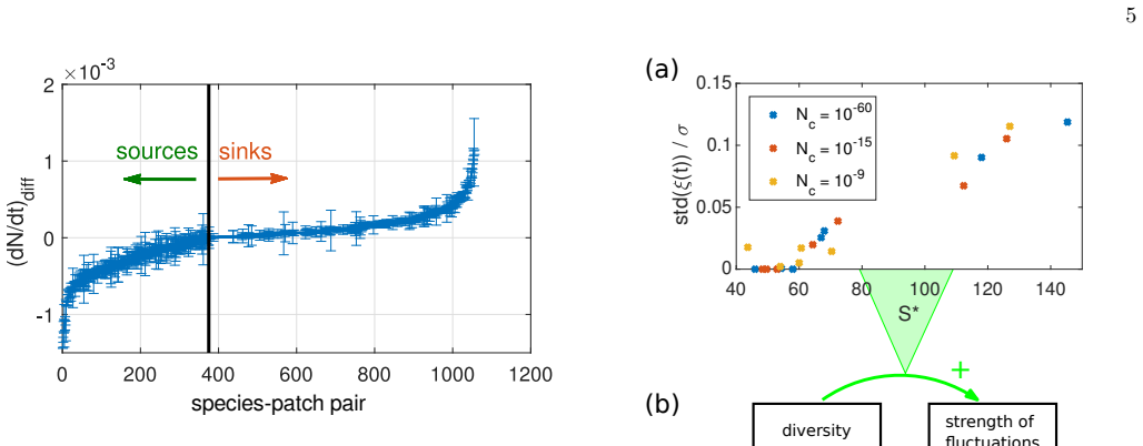
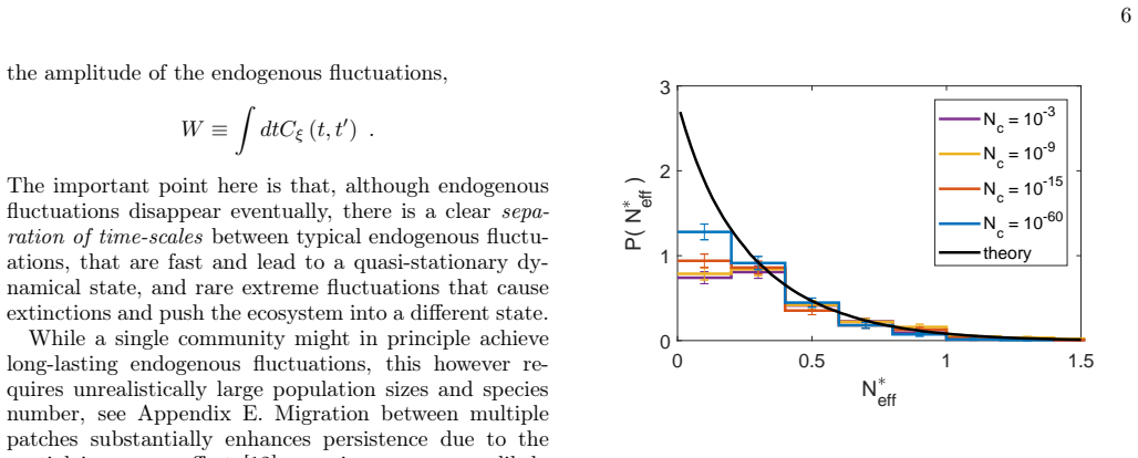
The load-bearing machinery is the dynamical mean-field theory (DMFT) mapping, which in the large-$S$ limit replaces the deterministic multi-species, multi-patch system by a single representative species in $M$ patches driven by a zero-mean Gaussian ecological noise $\xi_u(t)$, with the noise covariance fixed self-consistently by the species' own abundance correlations. From this mapping two derived quantities carry the argument: $W \equiv \int dt\, C_\xi(t,t')$, the integrated amplitude of the endogenous fluctuations, and $N^*_{\mathrm{eff}}$, an effective characteristic abundance constructed from the per-patch values $N^*_u$; together they set the activation exponent $a_{\mathrm{eff}}=2N^*_{\mathrm{eff}}/W$ in the extinction-time scaling. The framework also produces a self-consistent multivariate Gaussian distribution for the $N^*_u$, and the integral of that distribution over positive values gives a theoretical bound on the maximal long-term diversity. The spatial insurance is encoded in the exponent's factor $M$: extinction demands that all patches hit the cutoff, so the persistence time grows exponentially with patch number, provided the noise is asynchronous across patches and $W$ stays finite.
What would settle it
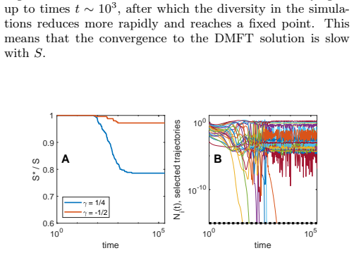
Compute the mean extinction time of a metacommunity as a function of $N_c$ for fixed $M$ and check whether $\log T_{\mathrm{ext}}$ grows linearly with $M\log(1/N_c)$: a slope that does not increase with $M$, or an integrated noise $W$ that grows with simulation time or as $D\to 0$, would falsify the scaling claim. A second check is direct: in the $M=8$, $\rho=0.95$ regime, if the surviving diversity $S^*/S$ keeps declining at times beyond $10^5$ instead of plateauing near the theoretical bound, the assumption of asynchronous noise between patches breaks.
Extended reading notes
Core claim
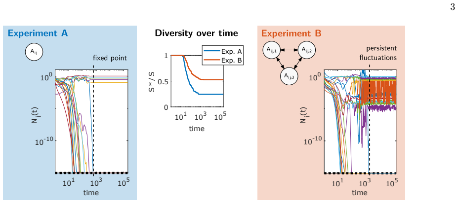
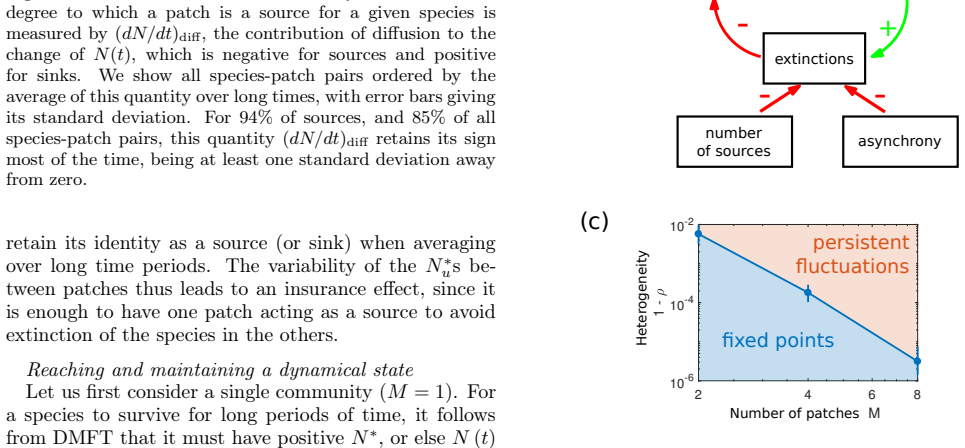
The central discovery is that high-diversity spatially extended systems, with small differences in conditions between locations, can enter a self-sustaining chaotic regime in which species abundances fluctuate over orders of magnitude and extinctions become rare rather than fatal. Extinction of a species requires its abundance to fall below a cutoff $N_c$ in every patch at once, so the mean time to extinction scales as $\tau (1/N_c)^{M a_{\mathrm{eff}}}$, where $M$ is the number of patches, $a_{\mathrm{eff}}=2N^*_{\mathrm{eff}}/W$, $W$ is the integrated amplitude of the endogenous fluctuations, and $N^*_{\mathrm{eff}}$ is an effective characteristic abundance across patches. Because the fluctuation noise is generated by the species themselves, diversity and fluctuation strength are locked in a feedback loop: losing species weakens the noise, which slows further extinctions. The paper shows that patches with higher characteristic abundance act as persistent sources, migration couples them to sinks, and this works even though the identity of a source patch is not imposed by the environment but emerges from interactions. In the same system with a single patch, the dynamics relax to a fixed point, which is why space and heterogeneity are the ingredients that convert an unstable high-diversity system into a long-lived fluctuating one.
Load-bearing premise
The analytical results assume that the integrated amplitude $W$ of the endogenous fluctuations stays finite as migration tends to zero and that the dynamical noise is uncorrelated between patches; if $W$ diverges or patches synchronize, the extinction-time scaling and the source-sink insurance argument collapse.
Editorial extensions
If this is right
- Whenever $M\ge 2$ patches are coupled by moderate migration ($d$ roughly at or below $10^{-1}$) and interaction coefficients differ slightly between patches, a high-diversity community should relax not to a fixed point but to a stationary chaotic state whose diversity is nearly constant over timescales of at least $10^5$.
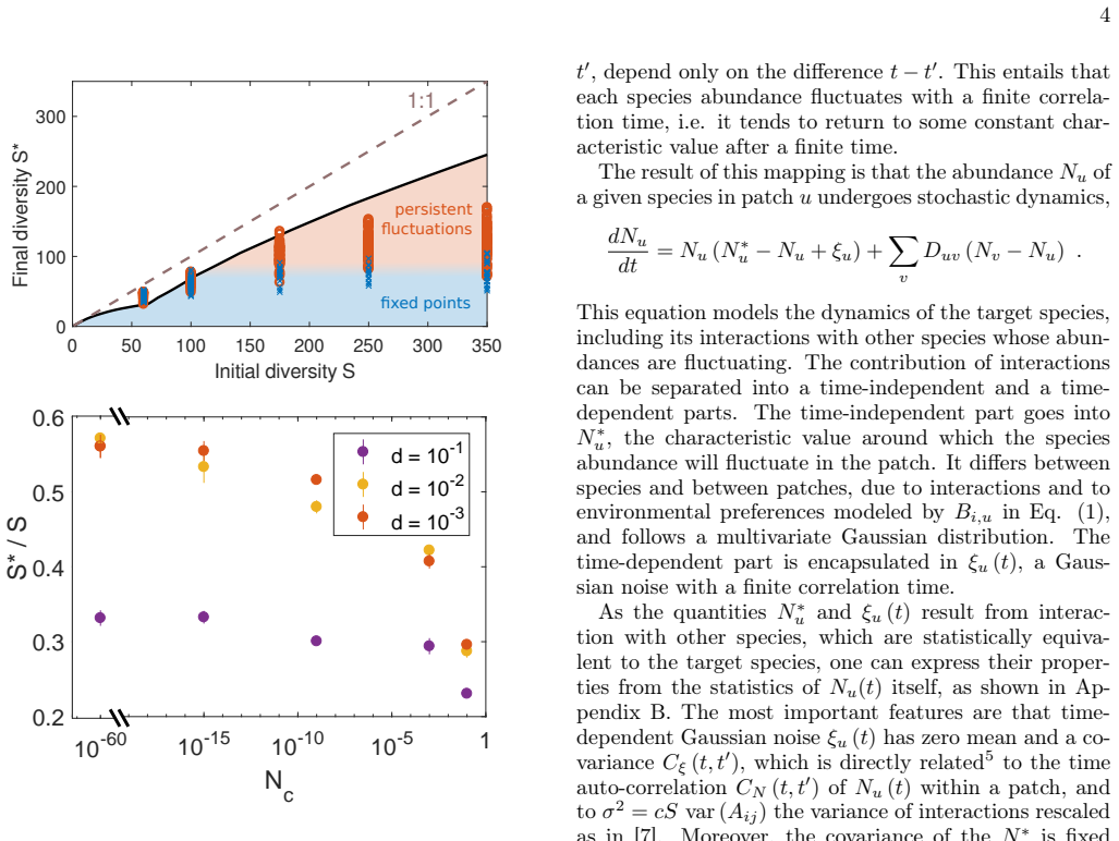
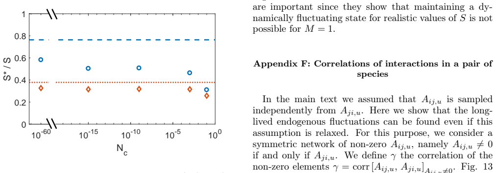
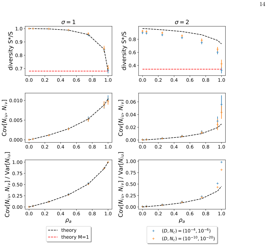
- The theoretical diversity bound derived from the distribution of $N^*_{\mathrm{eff}}$ implies that a fluctuating state can harbor more species than the same system at equilibrium; the bound is approached as the extinction cutoff $N_c$ decreases.
- Persistence time grows exponentially in the number of patches, as $(1/N_c)^{M a_{\mathrm{eff}}}$, so adding just a few patches with asynchronous dynamics vastly extends the lifetime of endogenous fluctuations.
- If patches synchronize—because migration is too strong or patch conditions are too similar—the insurance effect disappears and the system falls back to a low-diversity equilibrium, so synchrony is the control parameter for losing the fluctuating state.
- Experimental communities in multi-patch setups should show species-specific, unpredictable, asynchronous trajectories with long-lived diversity, whereas single-patch controls of identical composition converge to equilibrium.
Reading between the lines
- Beyond the paper: if the feedback loop is inverted by reducing spatial heterogeneity toward $\rho=1$, the theory predicts a delayed but accelerating extinction cascade, because diversity loss weakens exactly the noise that sustains the sources; this gives a testable dynamical route to biodiversity collapse that is distinct from deterministic loss of stability.
- Beyond the paper: the same DMFT machinery could be pointed at data by estimating $W$ and $N^*_{\mathrm{eff}}$ from time series of abundances in a multi-patch system, turning the paper's qualitative fingerprints—finite correlation time, asynchronous patches, source identity—into a quantitative classifier for whether observed fluctuations are endogenous.
- Beyond the paper: a microcosm experiment with the same species pool assembled in one well-mixed vessel and in several weakly coupled vessels with slightly different temperatures or resources should show the diversity plateau only in the coupled treatment; this would separate endogenous fluctuation persistence from purely environmental forcing.
Signed reviews
Editorial analysis
A structured set of objections, weighed in public.
Referee Report
Summary. The paper studies whether endogenous, interaction-driven fluctuations can persist for very long times in high-diversity ecological communities. It considers a Lotka-Volterra metacommunity with many species on multiple patches, with random interactions that vary slightly between patches, and an extinction cutoff Nc. Through simulations and dynamical mean-field theory (DMFT), the authors argue that a single well-mixed patch typically relaxes to a fixed point, whereas a spatially heterogeneous metacommunity with moderate migration can enter a chaotic, non-equilibrium state in which fluctuations and diversity maintain each other. The central theoretical claims are: (i) the effective stochastic dynamics of a representative species are governed by a noise ξ_u with finite integrated amplitude W, and with negligible cross-patch correlations; (ii) extinction times scale as τ(1/Nc)^(M a_eff), where the factor M arises from asynchronous fluctuations across patches; and (iii) DMFT predicts a diversity bound that is higher than the equilibrium (May-type) bound, matching simulations in many regimes. The simulations robustly show long-lived fluctuations at the selected parameter points, and the DMFT predictions for diversity and abundance correlations are compared with simulations over a range of parameters.
Significance. If the results hold, they constitute an important counterpoint to the classic view that large complex systems are unstable: a spatially extended system can maintain high diversity in a persistent non-equilibrium state, with fluctuations enabling coexistence far above the equilibrium bound. The paper is also valuable for its quantitative DMFT framework, which yields falsifiable predictions for diversity, fluctuation strength, and cross-patch correlations without fitting parameters to the simulation output. The comparison between theory and simulations is generally credible, and the authors are explicit about several limitations. However, the most distinctive quantitative claim -- the extinction-time scaling that justifies 'extremely long' persistence -- is not derived in this manuscript and rests on assumptions that are checked numerically only at parameter values far from the main simulations. Those gaps are load-bearing rather than cosmetic.
major comments (3)
- [Main text, 'Reaching and maintaining a dynamical state'; Appendix C] The central quantitative claim is the extinction-time scaling τ(1/Nc)^(M a_eff), stated in the main text and in Appendix C. However, Appendix C explicitly says 'We only present the result here; a full account will be given elsewhere.' Since this scaling is what converts finite-time simulations into the paper's headline assertion of 'extremely long' persistence, the result is currently a conjecture rather than a derivation. I ask the authors to either provide the derivation of Jmin = (2 xc / W) M N*_eff or explicitly present the scaling as a conjecture supported only by numerical evidence.
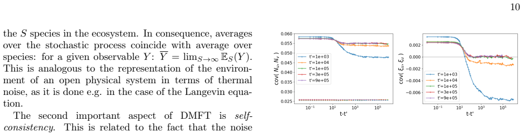
- [Appendix B, Fig. 7; Appendix C] The two assumptions that make the exponent M a_eff load-bearing are (i) finite integrated noise amplitude W and (ii) asynchrony, i.e. ξ_u(t) uncorrelated between patches for u≠v. The numerical check of these assumptions in Fig. 7 is performed at (S, M, ρ, d, Nc) = (400, 8, 0.95, 10^-10, 10^-15), whereas the main simulations use d = 10^-3 (Fig. 2) and D = 10^-4 (Figs. 5 and 6). No cross-patch dynamical-noise correlation is reported at those D values. Because the factor M in the exponent arises entirely from the asynchrony assumption, even a modest positive correlation between ξ_u and ξ_v would shorten the predicted persistence time by many orders of magnitude at small Nc. Please report the cross-patch ξ correlation and the decay of Cξ(t,t') at the parameter values used in the main figures.
- [Appendix D] Appendix D labels the finite-W assumption 'the main approximation (or limitation)' and notes that it breaks down if the noise develops long-lasting correlations in time. This assumption enters both the extinction-time exponent a = 2N*/W and the derivation of the D → 0 limit Nu = N*_u + O(D) used for the diversity bound. The paper's own limitation statement therefore flags exactly the quantity on which the headline result depends, while the numerical support for it is confined to an extreme parameter point. I request either a direct test of the finiteness of W (e.g., measurement of ∫dt Cξ(t,t') and its dependence on D) at the moderate-migration parameters of the main simulations, or an explicit statement that the diversity and persistence predictions are conditional on this assumption.
minor comments (4)
- [Appendix A] The sentence 'except in Appendix 13' should read 'except in Appendix F'.
- [Appendix C] The displayed definition of w is garbled: 'w≡− vuu√ 1/m ...' should be w = -sqrt((1/m) Σ_{u=1}^m (N*_u)^2), and the subsequent conditions on w should be stated with proper parentheses for readability.
- [Fig. 2 caption] The axis label 'Ni(t)' in the right panel contains stray commas; this appears to be a typesetting artifact and should be cleaned.
- [Main text, extinction threshold] The main text defines global extinction as the abundance falling below Nc in all patches, but the simulations in Fig. 10 use patch-wise extinctions with inward migration still allowed; the relation between these two implementations should be stated more explicitly in Appendix A.
Circularity Check
No circular reduction: the DMFT predictions are parameter-free and checked against direct simulations; only minor non-load-bearing self-citations are present.
full rationale
I find no step in the derivation chain that reduces to its own input by construction. The DMFT closure in Appendix D is solved self-consistently from the input statistics (mu, sigma, rho_uv, M, D, Nc) and then compared with independent simulations of the original Lotka-Volterra model (Figs. 2, 3, 6, 10), so the diversity and fluctuation predictions are not fitted outputs. The persistence-time scaling tau (1/Nc)^(M a_eff) is an application of large-deviation theory under two explicitly stated assumptions, finite W and asynchronous noise between patches; these are numerically checked rather than assumed into existence, and Appendix D itself labels finite W as 'the main approximation (or limitation)'. Appendix C's statement that 'a full account will be given elsewhere' is a deferral of proof, not a circular reuse of the conclusion. The self-citations to [14] (DMFT implementation) and [26] (single-patch stability threshold sigma_c = sqrt(2)) are real support for tools, but the paper's central claims are independently supported by its own simulations; hence the self-citations are minor and not load-bearing. No equation is equivalent to its inputs by definition, and no fitted parameter is renamed as a prediction.
Assumptions & free parameters
free parameters (4)
- migration rate d =
d=10^-3 in main runs
- patch interaction correlation rho =
rho=0.95 in main runs
- extinction cutoff Nc =
Nc=10^-15 in main runs; ranges 10^-60 to 10^-3 in parametric scans
- number of patches M =
M=8 in main runs; M=2 to 8 tested
assumptions (5)
- domain assumption DMFT mapping is exact in the S to infinity, C >> 1 limit for disordered interactions with product-measure disorder, and remains a controlled approximation at finite S.
- domain assumption The long-lived dynamical state is time-translation invariant (stationary) with finite correlation time, so two-time correlations depend only on time difference.
- domain assumption Fluctuations in different patches are asynchronous, with cross-patch dynamical noise xi_u(t) xi_v(t') negligible.
- ad hoc to paper The effective noise amplitude W = integral dt C_xi(t,t') remains finite as D -> 0+.
- domain assumption Rare extinction events can be described by large-deviation theory with a white-noise approximation for xi, yielding Arrhenius-like scaling.
Cite this review
Pith. "Pith review of Can endogenous fluctuations persist in high-diversity ecosystems?." pith.science (2026). https://pith.science/paper/HQLHBPAY
@misc{pith2026190803348,
  author       = {Pith},
  title        = {Pith review of: Can endogenous fluctuations persist in high-diversity ecosystems?},
  year         = {2026},
  howpublished = {\url{https://pith.science/paper/HQLHBPAY}},
  note         = {Machine review of arXiv:1908.03348}
}
read the original abstract
When can complex ecological interactions drive an entire ecosystem into a persistent non-equilibrium state, where species abundances keep fluctuating without going to extinction? We show that high-diversity spatially-extended systems, in which conditions vary somewhat between spatial locations, can exhibit chaotic dynamics which persist for extremely long times. We develop a theoretical framework, based on dynamical mean-field theory, to quantify the conditions under which these fluctuating states exist, and predict their properties. We uncover parallels with the persistence of externally-perturbed ecosystems, such as the role of perturbation strength, synchrony and correlation time. But uniquely to endogenous fluctuations, these properties arise from the species dynamics themselves, creating feedback loops between perturbation and response. A key result is that the fluctuation amplitude and species diversity are tightly linked, in particular fluctuations enable dramatically more species to coexist than at equilibrium in the very same system. Our findings highlight crucial differences between well-mixed and spatially-extended systems, with implications for experiments and their ability to reproduce natural dynamics. They shed light on the maintenance of biodiversity, and the strength and synchrony of fluctuations observed in natural systems.
Figures

Figures from the paper (10 more)

Reference graph
Works this paper leans on
-
[14]
Noise colour and the risk of population extinctions
Jörgen Ripa and Per Lundberg. Noise colour and the risk of population extinctions. Proceedings of the Royal Society of London. Series B: Biological Sciences , 263(1377):1751–1753, 1996
work page 1996
-
[27]
Ecological communities with Lotka-Volterra dynamics
Guy Bunin. Ecological communities with Lotka-Volterra dynamics. Physical Review E, 95(4), April 2017
work page 2017
-
[1]
Per Lundberg, Esa Ranta, Jörgen Ripa, and Veijo Kaitala. Population variability in space and time.Trends in Ecology & Evolution , 15(11):460–464, November 2000
work page 2000
-
[2]
These results are later explained in the theoretical analysis. All parameters for simulations are detailed in Appendix A. We focus on a meta-community which consists ofM patches (well-mixed systems) connected by migration, and isolated from the external world. We consider gener- alized Lotka-Volterra equations for the dynamics of the abundance Ni,u of spe...
work page 2020
-
[3]
On the relation be- tween temporal variability and persistence time in animal populations
Pablo Inchausti and John Halley. On the relation be- tween temporal variability and persistence time in animal populations. Journal of Animal Ecology , 72(6):899–908, November 2003
work page 2003
-
[4]
Chaos in a noisy world: New methods and evidence from time-series anal- ysis
Stephen Ellner and Peter Turchin. Chaos in a noisy world: New methods and evidence from time-series anal- ysis. The American Naturalist, 145(3):343–375, 1995
work page 1995
- [5]
-
[6]
Robert M. May. Biological populations with nonoverlap- ping generations: Stable points, stable cycles, and chaos. Science, 186(4164):645–647, 1974
work page 1974
Show all 30 references
-
[7]
J. C. Allen, W. M. Schaffer, and D. Rosko. Chaos reduces species extinction by amplifying local population noise. Nature, 364(6434):229–232, July 1993. 8
1993
-
[8]
Robert M. May. Will a large complex system be stable? Nature, 238(5364):413–414, 1972
1972
-
[9]
Berryman and J.A
A.A. Berryman and J.A. Millstein. Are ecological sys- tems chaotic — And if not, why not?Trends in Ecology & Evolution, 4(1):26–28, January 1989
1989
-
[10]
Roger Nisbet, Steve Blythe, Bill Gurney, Hans Metz, Kevin Stokes, Adam Lomnicki, and G.S. Mani. Avoid- ing chaos. Trends in Ecology & Evolution , 4(8):238–240, August 1989
1989
-
[11]
The average lifetime of a population in a varying environment.Journal of Theoretical Biology, 90(2):213–239, May 1981
Egbert Giles Leigh. The average lifetime of a population in a varying environment.Journal of Theoretical Biology, 90(2):213–239, May 1981
1981
-
[12]
Risks of Population Extinction from Demographic and Environmental Stochasticity and Random Catastrophes
Russell Lande. Risks of Population Extinction from Demographic and Environmental Stochasticity and Random Catastrophes. The American Naturalist , 142(6):911–927, 1993
1993
-
[13]
Biodiversity as spatial insurance in heterogeneous land- scapes
Michel Loreau, Nicolas Mouquet, and Andrew Gonzalez. Biodiversity as spatial insurance in heterogeneous land- scapes. Proceedings of the National Academy of Sciences, 100(22):12765–12770, 2003
2003
-
[15]
Felix Roy, Giulio Biroli, Guy Bunin, and Chiara Cam- marota. Numerical implementation of dynamical mean field theory for disordered systems: Application to the Lotka-Volterra model of ecosystems.Journal of Physics A: Mathematical and Theoretical , 2019
2019
-
[16]
Dominique Gravel, François Massol, and Mathew A. Leibold. Stability and complexity in model meta- ecosystems. Nature Communications, 7:12457, August 2016
2016
-
[17]
Graham and Ben G
Catherine H. Graham and Ben G. Weinstein. Towards a predictive model of species interaction beta diversity. Ecology Letters, 21(9):1299–1310, September 2018
2018
-
[18]
Generic assembly patterns in com- plex ecological communities.Proceedings of the National Academy of Sciences, 115(9):2156–2161, February 2018
Matthieu Barbier, Jean-François Arnoldi, Guy Bunin, and Michel Loreau. Generic assembly patterns in com- plex ecological communities.Proceedings of the National Academy of Sciences, 115(9):2156–2161, February 2018
2018
-
[19]
Carstensen, Malena Sabatino, Kristian Trø- jelsgaard, and Leonor Patricia C
Daniel W. Carstensen, Malena Sabatino, Kristian Trø- jelsgaard, and Leonor Patricia C. Morellato. Beta Diversity of Plant-Pollinator Networks and the Spa- tial Turnover of Pairwise Interactions. PLOS ONE , 9(11):e112903, November 2014
2014
-
[20]
Kordas, Christopher D.G
Rebecca L. Kordas, Christopher D.G. Harley, and Mary I. O’Connor. Community ecology in a warming world: The influence of temperature on interspecific in- teractions in marine systems. Journal of Experimen- tal Marine Biology and Ecology , 400(1-2):218–226, April 2011
2011
-
[21]
Biodiversity and ecosystem stability: A synthesis of underlying mech- anisms
Michel Loreau and Claire de Mazancourt. Biodiversity and ecosystem stability: A synthesis of underlying mech- anisms. Ecology Letters, 16(s1):106–115, 2013
2013
-
[22]
Chaos in random neural networks
Haim Sompolinsky, Andrea Crisanti, and Hans-Jurgen Sommers. Chaos in random neural networks. Physical Review Letters, 61(3):259, 1988
1988
-
[23]
John M. Halley. Ecology, evolution and 1f-noise.Trends in Ecology & Evolution , 11(1):33–37, January 1996
1996
-
[24]
The Bethe lattice spin glass revisited
Marc Mézard and Giorgio Parisi. The Bethe lattice spin glass revisited. The European Physical Journal B- Condensed Matter and Complex Systems , 20(2):217–233, 2001
2001
-
[25]
Stochasticmodels of population extinction.Trends in Ecology & Evolution , 25(11):643–652, November 2010
OtsoOvaskainenandBaruchMeerson. Stochasticmodels of population extinction.Trends in Ecology & Evolution , 25(11):643–652, November 2010
2010
-
[26]
How Colored Environmental Noise Affects Population Extinction
Alex Kamenev, Baruch Meerson, and Boris Shklovskii. How Colored Environmental Noise Affects Population Extinction. Physical Review Letters, 101(26):268103, De- cember 2008
2008
-
[28]
Stabilization of extensive fine-scale diversity by spatio-temporal chaos
M.T.Pearce, A.Agarwala, andD.S.Fisher. Stabilization of extensive fine-scale diversity by spatio-temporal chaos. bioRxiv (2019): 736215. 9 Appendix A: Model parameters used in simulations For convenient reference, this Appendix includes the parameters for all simulations. The m...
2019
-
[29]
On the other hand, ifN∗ 1 > 0, then we obtain the known result [11, 25] Jmin = 2xc W N∗ 1
If N∗ 1 < 0 the species is extinct. On the other hand, ifN∗ 1 > 0, then we obtain the known result [11, 25] Jmin = 2xc W N∗ 1 . The result for allM is a generalization of this result, of the form Jmin = 2xc W MN∗ eff . To describe the calculation ofN∗ eff, order the patches so t...
-
[30]
source” for patches whereN∗ u > 0, and “sink
Then N∗ eff = N∗ 1 and Jmin = 2xc W N∗ 1, so the result for M = 1 is reproduced. Another simple case is when there are M patches with identical carrying capacities N∗ u=1..M = N∗. Here{u}+ ={1,..,M} and w =−N∗. Then N∗ eff = N∗, and Jmin = 2xc W MN∗ eff = 2xc W MN∗. This result i...
Reviewed August 14, 2026 · model on record in the stance chip above.
Discussion (0). Continue with ORCID to comment.