REVIEW 5 major objections 8 minor 67 references
Saliency Maps are Ambiguous: Analysis of Logical Relations on First and Second Order Attributions
T0 review · 5 major / 8 minor · reviewed 2026-08-10 · deepseek-v4-flash
Pith's one-line read This paper claims that all 14 first-order saliency methods fail to rank logically necessary inputs above irrelevant baselines across all 21 tested logical dataset configurations, making saliency maps ambiguous as relevance rankings.
desk verdict Useful controlled benchmark and scenario rankings, but the central 'all methods fail' claim rests on NIB/GIB metrics that are stricter than the paper's own existential-check assumption. read the letter →
The pith
A machine-rendered reading of the paper's core claim, the machinery that carries it, and where it could break.
The reading
What carries the argument
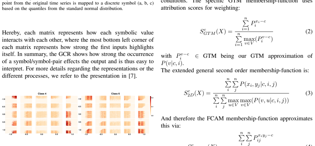
The central machinery is the ANDOR dataset framework, which generates fully controlled logical classification tasks with AND, OR, and XOR gates plus an irrelevant baseline block, so the complete set of minimally and maximally sufficient feature sets (R_min and R_max) is known for every sample. The paper measures each saliency method's ranking against those ground-truth information sets with the NIB and GIB metrics, and it applies the Global Coherence Representation (GCR), a symbolic global weight-aggregation model that turns local attribution scores into per-symbol, per-position class weights and can classify by weighted membership. The GCR's first-order GTM and second-order FCAM variants show whether saliency scores can function as class-relevance weights when inputs are fully omitted.
What would settle it
Retrain the same ANDOR models with a training objective that explicitly penalizes output sensitivity to baseline inputs, then re-apply NIB/GIB and the threshold-based masking. If no method still fails, the paper's conclusion that saliency maps are inherently ambiguous would be weakened; if the same failures persist in models with zero measured baseline sensitivity, the central claim would be strongly supported.
Extended reading notes
Core claim
Under the paper's Assumptions A-I, every one of the 14 first-order saliency methods violates at least one expected property in at least one of the 21 ANDOR dataset configurations: for some sample, a logically necessary input from the minimal information set R_min, or a globally relevant input from R_max, is scored below the highest baseline (irrelevant) input. The paper shows that failures concentrate in complementary-information cases and XOR gates, that information is sometimes leaked into masked inputs (DCA metrics), and that second-order aggregation (FCAM) recovers some global class differentiability that first-order scores lose. The authors conclude that saliency scores are ambiguous as local relevance rankings and that a weight-based interpretation, where the scores act as class-relevance weights and inputs can actually be omitted, is a more desirable verification direction.
Load-bearing premise
The load-bearing premise is that the ANDOR truth tables completely specify which inputs a correct explanation must mark as relevant, and that every relevant input must outscore every baseline input in the same sample; if the perfectly accurate model's real-valued output is genuinely sensitive to those baseline inputs, the reported failures may measure model complexity rather than explanation quality.
Editorial extensions
If this is right
- No analysed first-order saliency map can be read as a standalone ranking of feature importance; every method violates at least one of the paper's stated assumptions in at least one tested configuration.
- XOR-like or complementary-information settings are the hardest for all methods, supporting the paper's case that second-order attribution scores are needed to capture joint input relevance.
- Methods with good local information capture, such as IntegratedGradients, do not necessarily produce globally comparable scores, so local and global interpretations of the same method can disagree.
- A weight-based interpretation such as the GCR can preserve class differentiability even when first-order rankings fail, suggesting that input-omitting interpretations are more promising than raw heatmap rankings.
Reading between the lines
- If the reported failures partly reflect real-valued model outputs rather than explanation-method flaws, then the NIB/GIB metrics may conflate explanation quality with model complexity; a cleaner test would measure NIB/GIB on models with explicitly zero sensitivity to baseline inputs.
- The scenario ranking suggests a practical selector: for AND-OR-like tasks, perturbation-based methods may be defensible, while XOR-heavy tasks should probably receive higher-order explanations by default.
- A direct extension would replace the fixed 'highest baseline score' threshold with per-method calibrated thresholds; if ranking conclusions change, part of the observed ambiguity is a threshold artifact rather than an inherent property of saliency scores.
Editorial analysis
A structured set of objections, weighed in public.
Referee Report
Summary. The paper extends the authors' ANDOR logical dataset framework to evaluate the reliability of saliency maps. It trains CNN and Transformer models on 21 ANDOR dataset configurations and applies 14 first-order and 4 second-order attribution methods, spanning 336 experiments and 404,880 trained models. The central empirical claim is that no analysed saliency method consistently ranks all logically necessary inputs above a non-informative baseline; IntegratedGradients, LRP-Rollout, and Attention are identified as the best, yet still imperfect. The paper also proposes the Global Coherence Representation (GCR) as a weight-based, global interpretation and evaluation approach, and it provides per-scenario rankings of methods across multiple metrics (NIB, GIB, logical accuracy, DCA, correlation, GCR fidelity).
Significance. If the central negative result holds, it is an important contribution to XAI, suggesting fundamental limits of first-order attribution maps even in fully controlled logical tasks with externally defined ground truth. The scale of the experiments and the explicit logical ground truth are strengths, as is the open-source code. The paper also offers practical per-scenario comparisons of 14 first-order and 4 second-order methods, which is valuable. However, the validity of the main claim depends on the strictness of the NIB/GIB metrics and on the assumption that a 100%-accurate model's decision behavior is fully reducible to the logical formula. The GCR proposal is interesting but requires additional validation to avoid circularity.
major comments (5)
- [IV-C, III-A, III-C] The NIB and GIB definitions implement a universal quantification over all minimal/maximal sets, which is stronger than the paper's own Assumption B and the Section III-A statement that the ranking should "match one possible reasoning r in Rd_min". For an OR-positive sample with two positive inputs, if one positive input scores above the baseline and the other below, NIB counts the sample as failed even though a sufficient minimal set is correctly ranked. Similarly, GIB counts every Rd_max input that falls below the baseline as a miss. This inflates failure rates and directly drives the central "all methods fail" claim. Please report an existential variant (e.g., the percentage of samples with at least one fully correct minimal set) and a redundant-aware variant, and clarify which of the paper's claims each metric supports.
- [V-A, Table II] The per-method interpretation mode (AsIs/Cutoff/Absolute) is selected based on the NIB metric on the same test data used for the reported NIB results. This is a selection-on-target procedure: methods with more flexible post-processing benefit, and the reported NIB values are optimistically biased. While this does not rescue any method to a perfect score, it affects the cross-method ranking (Table IV) and the claim that IntegratedGradients is best at information capturing. Please select modes on a held-out validation set or pre-specify them per method, and report results for all three modes so readers can assess sensitivity.
- [V-E, VI-B] The paper's own correlation analysis shows that baseline inputs alter model outputs: "changing irrelevant inputs will likely (slightly) change the numeric output." This means the 100%-accurate models are not exact implementations of the ANDOR formula, so NIB/GIB failures could measure model sensitivity to baseline inputs rather than explanation quality. The Limitations section acknowledges that the model output does not have zero error, but it asserts that relevant inputs should still be scored highest because inputs are independent. This assertion needs quantitative support: for example, report the effect size of baseline inputs on output logits relative to relevant inputs, or verify that the NIB/GIB failures persist for models with near-zero loss.
- [V-E, Figure 12] The text and Figure 12 report "significant (p < 0.5) Pearson correlations". If p<0.5 is literal, this is not a valid significance threshold and invalidates the correlation analysis, since nearly all correlations would be "significant". If it is a typo for p<0.05, the percentage-of-significant-cases panel changes substantially. Please correct the threshold and recompute the correlation results.
- [III-D, V-F] The GCR is both proposed as an interpretation framework and used as an evaluation tool via GCR Fidelity and tGCR Fidelity. The membership functions (Eq. 2 and Eq. 4) are defined by the authors without an axiomatic justification, and using them to evaluate saliency methods is partly circular. High GCR fidelity may reflect the averaging properties of the GCR rather than the quality of the saliency scores. Please validate the GCR against independent aggregation schemes (e.g., simple linear probes or other global aggregation baselines) and clearly state which conclusions depend on the GCR's specific assumptions.
minor comments (8)
- [III-C] The assumptions are labeled (A), (B), (C), (D), (E), (F), (H), (I), skipping (G); please renumber or add a missing item.
- [Abstract] Typo: "confirmations bias" should be "confirmation bias".
- [IV-C] The Full-DCA definition uses "N rB" which is undefined.
- [V-E] The text refers to Assumption I when the relevant assumption on undesired correlations is Assumption H; please fix the cross-reference.
- [III-F] The dataset size for 2inQuaternary is given as 65526; it should be 65536 (=4^8).
- [Appendix Figure 18] The caption "verage Full-DCA" should be "Average Full-DCA".
- [V-H] Table III labels GCR FCAM/GTM values as "Acc." while the text describes them as "global differentiability"; please clarify whether these are accuracies or normalized scores.
- [II] The related work could more explicitly summarize how this work differs from the authors' previous [4] in terms of new datasets, metrics, and second-order methods.
Circularity Check
No significant circularity: NIB/GIB are compared to an externally defined truth-table ground truth, and the GCR self-citations are descriptive rather than load-bearing.
full rationale
The central empirical claim is not circular: NIB/GIB compare saliency-score rankings against Rd_min and Rd_max, which are defined from the ANDOR truth tables (Section III-A) and the baseline-input rule (Assumption E), independently of any saliency method. The all-methods-fail result is therefore a substantive finding relative to that external ground truth, not an identity. The paper's self-citations to [4] and [5,6,7] are descriptive rather than load-bearing: the ANDOR formalization and assumptions are restated in Sections III-A and III-C, and the GCR is specified by explicit membership equations (Eqs. 1-4), so the evaluation does not reduce to an unverified citation. The disclosed per-method selection of score interpretation mode (AsIs/Cutoff/Absolute) using the NIB metric is a transparency concern and could inflate relative rankings, but it is not a hidden circular step because it is stated and because the central failure claim holds even under the best mode. The closest issue is that NIB/GIB quantify exhaustively over all minimal/maximal sets, which conflicts with the existential 'matches one possible reasoning r in Rd_min' wording and Assumption B in redundant scenarios; however, this is a validity/interpretation mismatch between the metric and the paper's own assumptions, not an equivalence-by-construction between the ground truth and the output, so it does not make the derivation circular. Overall, the paper is self-contained against an external logical benchmark.
Assumptions & free parameters
free parameters (3)
- Per-method saliency interpretation mode (AsIs/Cutoff/Absolute) =
See Table II (e.g., IntegratedGradients: Absolute, LRP-Full: Cutoff)
- Full-DCA threshold factors =
1.0, 0.8, 0.5
- GCR/SAX hyperparameters (alphabet size v, symbol mapping) =
Not stated in the paper; only referenced via code
assumptions (4)
- domain assumption The ANDOR truth-table sets Rd_min and Rd_max are the complete set of valid model reasonings for each dataset (Section III-A and III-G).
- domain assumption Baseline inputs are truly class-irrelevant, and any relevant input must be scored above the highest baseline input per sample (Assumptions D and E, Section III-C).
- domain assumption Saliency score ordering is meaningful and scores are globally comparable across samples (Assumptions A and I, Section III-C).
- ad hoc to paper The GCR membership functions (Equations 2 and 4) are a valid way to interpret attribution scores as classification weights.
Cite this review
Pith. "Pith review of Saliency Maps are Ambiguous: Analysis of Logical Relations on First and Second Order Attributions." pith.science (2026). https://pith.science/paper/HQYFOHSL
@misc{pith2026250114136,
  author       = {Pith},
  title        = {Pith review of: Saliency Maps are Ambiguous: Analysis of Logical Relations on First and Second Order Attributions},
  year         = {2026},
  howpublished = {\url{https://pith.science/paper/HQYFOHSL}},
  note         = {Machine review of arXiv:2501.14136}
}
read the original abstract
Recent work uncovered potential flaws in \eg attribution or heatmap based saliency methods. A typical flaw is a confirmations bias, where the scores are compared to human expectation. Since measuring the quality of saliency methods is hard due to missing ground truth model reasoning, finding general limitations is also hard. This is further complicated, because masking-based evaluation on complex data can easily introduce a bias, as most methods cannot fully ignore inputs. In this work, we extend our previous analysis on the logical dataset framework ANDOR, where we showed that all analysed saliency methods fail to grasp all needed classification information for all possible scenarios. Specifically, this paper extends our previous work using analysis on more datasets, in order to better understand in which scenarios the saliency methods fail. Further, we apply the Global Coherence Representation as an additional evaluation method in order to enable actual input omission.
Figures


Figures from the paper (18 more)




Reference graph
Works this paper leans on
-
[1]
Sanity checks for saliency maps,
J. Adebayo, J. Gilmer, M. Muelly, I. Goodfellow, M. Hardt, and B. Kim, “Sanity checks for saliency maps,” Advances in neural information processing sys- tems, vol. 31, 2018
work page 2018
-
[2]
Logic Traps in Evaluating Attribution Scores
Y . Ju, Y . Zhang, Z. Yang, Z. Jiang, K. Liu, and J. Zhao, “Logic traps in evaluating attribution scores,” arXiv preprint arXiv:2109.05463, 2021
work page Pith review arXiv 2021
-
[3]
Evaluation of post-hoc interpretability methods in time- series classification,
H. Turb ´e, M. Bjelogrlic, C. Lovis, and G. Mengaldo, “Evaluation of post-hoc interpretability methods in time- series classification,” Nature Machine Intelligence, vol. 5, no. 3, pp. 250–260, 2023
work page 2023
-
[4]
Saliency methods are encoders: Analysing logical relations towards interpreta- tion,
L. Schwenke and M. Atzmueller, “Saliency methods are encoders: Analysing logical relations towards interpreta- tion,” 2024
work page 2024
-
[5]
L. Schwenke and M. Atzmueller, “Constructing global coherence representations: Identifying interpretability and coherences of transformer attention in time series data,” in Proc. IEEE International Conference on Data Science and Advanced Analytics (DSAA) , IEEE, 2021
work page 2021
-
[6]
Abstracting local transformer attention for enhancing interpretability on time series data.,
L. Schwenke and M. Atzmueller, “Abstracting local transformer attention for enhancing interpretability on time series data.,” in LWDA, pp. 205–218, 2021
work page 2021
-
[7]
Extracting Interpretable Local and Global Representations from Attention on Time Series
L. Schwenke and M. Atzmueller, “Extracting inter- pretable local and global representations from attention on time series,” arXiv preprint arXiv:2312.11466 , 2023
work page Pith review arXiv 2023
-
[8]
Molnar, Interpretable machine learning
C. Molnar, Interpretable machine learning . Lulu. com, 2020
2020
Show all 67 references
-
[9]
Joint shapley values: a measure of joint feature importance,
C. Harris, R. Pymar, and C. Rowat, “Joint shapley values: a measure of joint feature importance,” arXiv preprint arXiv:2107.11357, 2021
2021 arXiv
-
[10]
Shapley residuals: Quantifying the limits of the shapley value for explanations,
I. Kumar, C. Scheidegger, S. Venkatasubramanian, and S. Friedler, “Shapley residuals: Quantifying the limits of the shapley value for explanations,” Advances in Neural Information Processing Systems , vol. 34, pp. 26598– 26608, 2021
2021
-
[11]
Faith-shap: The faithful shapley interaction index,
C.-P. Tsai, C.-K. Yeh, and P. Ravikumar, “Faith-shap: The faithful shapley interaction index,” Journal of Ma- chine Learning Research, vol. 24, no. 94, pp. 1–42, 2023
2023
-
[12]
Disentan- gling interactions and dependencies in feature attribu- tion,
G. K ¨onig, E. G ¨unther, and U. von Luxburg, “Disentan- gling interactions and dependencies in feature attribu- tion,” arXiv preprint arXiv:2410.23772 , 2024
2024 arXiv
-
[13]
Shap-iq: Unified approximation of any-order shapley interactions,
F. Fumagalli, M. Muschalik, P. Kolpaczki, E. H ¨ullermeier, and B. Hammer, “Shap-iq: Unified approximation of any-order shapley interactions,” Advances in Neural Information Processing Systems , vol. 36, 2024
2024
-
[14]
Interpreting multivariate shapley interactions in dnns,
H. Zhang, Y . Xie, L. Zheng, D. Zhang, and Q. Zhang, “Interpreting multivariate shapley interactions in dnns,” in Proceedings of the AAAI Conference on Artificial Intelligence, vol. 35, pp. 10877–10886, 2021
2021
-
[15]
How does this interaction affect me? interpretable attribution for feature interactions,
M. Tsang, S. Rambhatla, and Y . Liu, “How does this interaction affect me? interpretable attribution for feature interactions,” Advances in neural information processing systems, vol. 33, pp. 6147–6159, 2020
2020
-
[16]
Explaining explanations: Axiomatic feature interactions for deep net- works,
J. D. Janizek, P. Sturmfels, and S.-I. Lee, “Explaining explanations: Axiomatic feature interactions for deep net- works,” Journal of Machine Learning Research , vol. 22, no. 104, pp. 1–54, 2021
2021
-
[18]
Ma- chine learning interpretability: A survey on methods and metrics,
D. V . Carvalho, E. M. Pereira, and J. S. Cardoso, “Ma- chine learning interpretability: A survey on methods and metrics,” Electronics, vol. 8, no. 8, p. 832, 2019
2019
-
[19]
An experimental study of quantitative evaluations on saliency methods,
X.-H. Li, Y . Shi, H. Li, W. Bai, C. C. Cao, and L. Chen, “An experimental study of quantitative evaluations on saliency methods,” in Proceedings of the 27th ACM sigkdd conference on knowledge discovery & data min- ing, pp. 3200–3208, 2021
2021
-
[20]
The (un) reliability of saliency methods,
P.-J. Kindermans, S. Hooker, J. Adebayo, M. Alber, K. T. Sch ¨utt, S. D ¨ahne, D. Erhan, and B. Kim, “The (un) reliability of saliency methods,” Explainable AI: Interpreting, explaining and visualizing deep learning , pp. 267–280, 2019
2019
-
[21]
Do input gradients highlight discriminative features?,
H. Shah, P. Jain, and P. Netrapalli, “Do input gradients highlight discriminative features?,” Advances in Neural Information Processing Systems, vol. 34, pp. 2046–2059, 2021
2021
-
[22]
Investigating sanity checks for saliency maps with image and text classification,
N. Kokhlikyan, V . Miglani, B. Alsallakh, M. Martin, and O. Reblitz-Richardson, “Investigating sanity checks for saliency maps with image and text classification,” arXiv preprint arXiv:2106.07475, 2021
2021 arXiv
-
[23]
When explanations lie: Why many modified bp attributions fail,
L. Sixt, M. Granz, and T. Landgraf, “When explanations lie: Why many modified bp attributions fail,” in Interna- tional conference on machine learning , pp. 9046–9057, PMLR, 2020
2020
-
[24]
Towards faithfully inter- pretable nlp systems: How should we define and evaluate faithfulness?,
A. Jacovi and Y . Goldberg, “Towards faithfully inter- pretable nlp systems: How should we define and evaluate faithfulness?,” arXiv preprint arXiv:2004.03685 , 2020
2004 arXiv
-
[25]
On baselines for local feature attributions,
J. Haug, S. Z ¨urn, P. El-Jiz, and G. Kasneci, “On baselines for local feature attributions,” arXiv preprint arXiv:2101.00905, 2021
2021 arXiv
-
[26]
Visualizing the impact of feature attribution baselines,
P. Sturmfels, S. Lundberg, and S.-I. Lee, “Visualizing the impact of feature attribution baselines,” Distill, vol. 5, no. 1, p. e22, 2020
2020
-
[27]
A benchmark for interpretability methods in deep neural networks,
S. Hooker, D. Erhan, P.-J. Kindermans, and B. Kim, “A benchmark for interpretability methods in deep neural networks,” Advances in neural information processing systems, vol. 32, 2019
2019
-
[28]
A consistent and efficient evalua- tion strategy for attribution methods,
Y . Rong, T. Leemann, V . Borisov, G. Kasneci, and E. Kasneci, “A consistent and efficient evalua- tion strategy for attribution methods,” arXiv preprint arXiv:2202.00449, 2022
2022 arXiv
-
[29]
Geometric remove-and-retrain (goar): Coordinate-invariant explain- able ai assessment,
Y .-H. Park, J. Seo, B. Park, S. Lee, and J. Jo, “Geometric remove-and-retrain (goar): Coordinate-invariant explain- able ai assessment,” in XAI in Action: Past, Present, and Future Applications, 2023
2023
-
[30]
Learning global pairwise interactions with bayesian neural networks,
T. Cui, P. Marttinen, and S. Kaski, “Learning global pairwise interactions with bayesian neural networks,” in ECAI 2020, pp. 1087–1094, IOS Press, 2020
2020
-
[31]
Fooling lime and shap: Adversarial attacks on post hoc explanation methods,
D. Slack, S. Hilgard, E. Jia, S. Singh, and H. Lakkaraju, “Fooling lime and shap: Adversarial attacks on post hoc explanation methods,” in Proceedings of the AAAI/ACM Conference on AI, Ethics, and Society , pp. 180–186, 2020
2020
-
[32]
Shapley values for feature selection: The good, the bad, and the axioms,
D. Fryer, I. Str ¨umke, and H. Nguyen, “Shapley values for feature selection: The good, the bad, and the axioms,” Ieee Access, vol. 9, pp. 144352–144360, 2021
2021
-
[33]
Show me what you’re looking for: Visualizing abstracted transformer attention for enhancing their local interpretability on time series data,
L. Schwenke and M. Atzmueller, “Show me what you’re looking for: Visualizing abstracted transformer attention for enhancing their local interpretability on time series data,” in Proc. FLAIRS, (North Miami Beach, FL, USA), pp. 402–407, 2021
2021
-
[34]
A survey on neural network interpretability,
Y . Zhang, P. Tiˇno, A. Leonardis, and K. Tang, “A survey on neural network interpretability,”IEEE Transactions on Emerging Topics in Computational Intelligence , vol. 5, no. 5, pp. 726–742, 2021
2021
-
[35]
Logic-based explainability in machine learning,
J. Marques-Silva, “Logic-based explainability in machine learning,” in Reasoning Web. Causality, Explanations and Declarative Knowledge: 18th International Summer School 2022, Berlin, Germany, September 27–30, 2022, Tutorial Lectures, pp. 24–104, Springer, 2023
2022
-
[36]
Revisit fuzzy neural network: bridging the gap between fuzzy logic and deep learning,
L. Fan, “Revisit fuzzy neural network: bridging the gap between fuzzy logic and deep learning,” tech. rep., Technical Report, 2017
2017
-
[37]
Neural-symbolic learning and reasoning: A survey and interpretation,
A. d. Garcez, S. Bader, H. Bowman, L. C. Lamb, L. de Penning, B. Illuminoo, H. Poon, and C. G. Za- verucha, “Neural-symbolic learning and reasoning: A survey and interpretation,” Neuro-Symbolic Artificial In- telligence: The State of the Art , vol. 342, no. 1, p. 327, 2022
2022
-
[38]
Logical expla- nations for deep relational machines using relevance information,
A. Srinivasan, L. Vig, and M. Bain, “Logical expla- nations for deep relational machines using relevance information,” Journal of Machine Learning Research , vol. 20, no. 130, pp. 1–47, 2019
2019
-
[39]
Meaningful explanations of black box ai decision systems,
D. Pedreschi, F. Giannotti, R. Guidotti, A. Monreale, S. Ruggieri, and F. Turini, “Meaningful explanations of black box ai decision systems,” in Proceedings of the AAAI conference on artificial intelligence , vol. 33, pp. 9780–9784, 2019
2019
-
[40]
Evaluating the correctness of explainable ai algorithms for classification,
O. Yalcin, X. Fan, and S. Liu, “Evaluating the correctness of explainable ai algorithms for classification,” arXiv preprint arXiv:2105.09740, 2021
2021 arXiv
-
[41]
Evaluation of post-hoc xai approaches through synthetic tabular data,
J. Tritscher, M. Ring, D. Schlr, L. Hettinger, and A. Hotho, “Evaluation of post-hoc xai approaches through synthetic tabular data,” in Foundations of In- telligent Systems: 25th International Symposium, ISMIS 2020, Graz, Austria, September 23–25, 2020, Proceed- ings, pp. 422–...
2020
-
[42]
Evaluating feature attribution: An information-theoretic perspective,
Y . Rong, T. Leemann, V . Borisov, G. Kasneci, and E. Kasneci, “Evaluating feature attribution: An information-theoretic perspective,” CoRR, 2022
2022
-
[43]
Sanity checks for saliency metrics,
R. Tomsett, D. Harborne, S. Chakraborty, P. Gurram, and A. Preece, “Sanity checks for saliency metrics,” in Proceedings of the AAAI conference on artificial intelligence, vol. 34, pp. 6021–6029, 2020
2020
-
[44]
Metrics for saliency map evaluation of deep learning explanation methods,
T. Gomez, T. Fr ´eour, and H. Mouch `ere, “Metrics for saliency map evaluation of deep learning explanation methods,” in International Conference on Pattern Recog- nition and Artificial Intelligence , pp. 84–95, Springer, 2022
2022
-
[45]
Explaining deep neural networks: A survey on the global interpretation methods,
R. Saleem, B. Yuan, F. Kurugollu, A. Anjum, and L. Liu, “Explaining deep neural networks: A survey on the global interpretation methods,” Neurocomputing, vol. 513, pp. 165–180, 2022
2022
-
[46]
A Symbolic Representation of Time Series, with Implications for Streaming Algorithms,
J. Lin, E. Keogh, S. Lonardi, and B. Chiu, “A Symbolic Representation of Time Series, with Implications for Streaming Algorithms,” in Proc. 8th ACM SIGMOD Workshop on Research Issues in Data Mining and Knowl- edge Discovery, (New York, NY , USA), pp. 2–11, ACM, 2003
2003
-
[47]
Experiencing SAX: A Novel Symbolic Representation of Time Series,
J. Lin, E. Keogh, L. Wei, and S. Lonardi, “Experiencing SAX: A Novel Symbolic Representation of Time Series,” Data Mining and Knowledge Discovery , vol. 15, no. 2, pp. 107–144, 2007
2007
-
[48]
Explainable artificial intelli- gence (xai) on timeseries data: A survey,
T. Rojat, R. Puget, D. Filliat, J. Del Ser, R. Gelin, and N. D ´ıaz-Rodr´ıguez, “Explainable artificial intelli- gence (xai) on timeseries data: A survey,” arXiv preprint arXiv:2104.00950, 2021
2021 arXiv
-
[49]
Explanation-aware feature selection using symbolic time series abstraction: approaches and experiences in a petro-chemical production context,
M. Atzmueller, N. Hayat, A. Schmidt, and B. Kl ¨opper, “Explanation-aware feature selection using symbolic time series abstraction: approaches and experiences in a petro-chemical production context,” in 2017 IEEE 15th International Conference on Industrial Informatics (INDIN),...
2017
-
[50]
Imbalanced-learn: A python toolbox to tackle the curse of imbalanced datasets in machine learning,
G. Lema ˆıtre, F. Nogueira, and C. K. Aridas, “Imbalanced-learn: A python toolbox to tackle the curse of imbalanced datasets in machine learning,” Journal of Machine Learning Research , vol. 18, no. 17, pp. 1–5, 2017
2017
-
[51]
Transformers in time series: A survey,
Q. Wen, T. Zhou, C. Zhang, W. Chen, Z. Ma, J. Yan, and L. Sun, “Transformers in time series: A survey,” arXiv preprint arXiv:2202.07125, 2022
2022 arXiv
-
[52]
Grad-cam: Visual explanations from deep networks via gradient-based localization,
R. R. Selvaraju, M. Cogswell, A. Das, R. Vedantam, D. Parikh, and D. Batra, “Grad-cam: Visual explanations from deep networks via gradient-based localization,” in Proceedings of the IEEE international conference on computer vision, pp. 618–626, 2017
2017
-
[53]
Deep residual learning for image recognition,
K. He, X. Zhang, S. Ren, and J. Sun, “Deep residual learning for image recognition,” in Proceedings of the IEEE conference on computer vision and pattern recog- nition, pp. 770–778, 2016
2016
-
[54]
Attention is all you need,
A. Vaswani, N. Shazeer, N. Parmar, J. Uszkoreit, L. Jones, A. N. Gomez, Ł. Kaiser, and I. Polosukhin, “Attention is all you need,” Advances in neural informa- tion processing systems , vol. 30, 2017
2017
-
[55]
Transformer inter- pretability beyond attention visualization,
H. Chefer, S. Gur, and L. Wolf, “Transformer inter- pretability beyond attention visualization,” in Proceed- ings of the IEEE/CVF conference on computer vision and pattern recognition, pp. 782–791, 2021
2021
-
[56]
On pixel-wise explanations for non-linear classifier decisions by layer-wise relevance propagation,
S. Bach, A. Binder, G. Montavon, F. Klauschen, K.- R. M ¨uller, and W. Samek, “On pixel-wise explanations for non-linear classifier decisions by layer-wise relevance propagation,” PloS one, vol. 10, no. 7, p. e0130140, 2015
2015
-
[57]
Quantifying attention flow in transformers,
S. Abnar and W. Zuidema, “Quantifying attention flow in transformers,” arXiv preprint arXiv:2005.00928, 2020
2005 arXiv
-
[58]
Axiomatic at- tribution for deep networks,
M. Sundararajan, A. Taly, and Q. Yan, “Axiomatic at- tribution for deep networks,” in International conference on machine learning , pp. 3319–3328, PMLR, 2017
2017
-
[59]
Captum: A unified and generic model interpretability library for pytorch,
N. Kokhlikyan, V . Miglani, M. Martin, E. Wang, B. Alsallakh, J. Reynolds, A. Melnikov, N. Kliushkina, C. Araya, S. Yan, et al., “Captum: A unified and generic model interpretability library for pytorch,” arXiv preprint arXiv:2009.07896, 2020
2009 arXiv
-
[60]
Learning important features through propagating activation differ- ences,
A. Shrikumar, P. Greenside, and A. Kundaje, “Learning important features through propagating activation differ- ences,” in International conference on machine learning , pp. 3145–3153, PMLR, 2017
2017
-
[61]
Visualizing and understand- ing convolutional networks,
M. D. Zeiler and R. Fergus, “Visualizing and understand- ing convolutional networks,” in Computer Vision–ECCV 2014: 13th European Conference, Zurich, Switzerland, September 6-12, 2014, Proceedings, Part I 13 , pp. 818– 833, Springer, 2014
2014
-
[62]
Pytorch library for cam methods
J. Gildenblat and contributors, “Pytorch library for cam methods.” https://github.com/jacobgil/pytorch-grad-cam, 2021
2021
-
[63]
Grad-cam++: Generalized gradient- based visual explanations for deep convolutional net- works,
A. Chattopadhay, A. Sarkar, P. Howlader, and V . N. Balasubramanian, “Grad-cam++: Generalized gradient- based visual explanations for deep convolutional net- works,” in 2018 IEEE winter conference on applications of computer vision (WACV) , pp. 839–847, IEEE, 2018
2018
-
[64]
A unified approach to interpreting model predictions,
S. M. Lundberg and S.-I. Lee, “A unified approach to interpreting model predictions,” Advances in neural information processing systems , vol. 30, 2017
2017
-
[65]
On the effects of non-normality on the distribution of the sample product-moment correlation coefficient,
C. J. Kowalski, “On the effects of non-normality on the distribution of the sample product-moment correlation coefficient,” Journal of the Royal Statistical Society: Series C (Applied Statistics) , vol. 21, no. 1, pp. 1–12, 1972
1972
-
[66]
Random forests,
L. Breiman, “Random forests,” Machine learning , vol. 45, pp. 5–32, 2001
2001
-
[67]
Unmasking clever hans predictors and assessing what machines really learn,
S. Lapuschkin, S. W ¨aldchen, A. Binder, G. Montavon, W. Samek, and K.-R. M ¨uller, “Unmasking clever hans predictors and assessing what machines really learn,” Nature communications, vol. 10, no. 1, p. 1096, 2019
2019
-
[68]
Revisiting sanity checks for saliency maps,
G. Yona and D. Greenfeld, “Revisiting sanity checks for saliency maps,” arXiv preprint arXiv:2110.14297 , 2021. APPENDIX In the following, we provide addition plots, showing the results when considering all trained models, to provide further results supporting our discussion. ...
2021 arXiv
Reviewed August 10, 2026 · model on record in the stance chip above.
Discussion (0). Continue with ORCID to comment.