REVIEW 3 major objections 6 minor 18 references
Revealing hidden correlations from complex spatial distributions: Adjacent Correlation Analysis
T0 review · 3 major / 6 minor · reviewed 2026-08-07 · deepseek-v4-flash
Pith's one-line read Local spatial correlations add up to a predictive vector field
desk verdict A new and useful exploratory visualization for local spatial correlations, but the claimed equivalence to dynamical-systems vector fields is an overreach and the method parameters need specification. read the letter →
The pith
A machine-rendered reading of the paper's core claim, the machinery that carries it, and where it could break.
The reading
What carries the argument
The load-bearing construction is the spin-2 correlation vector. For each location in the parameter plot, the method finds all measured points whose values fall in a small neighborhood of that location; for each such point it evaluates the spatial gradient of the two quantities, $\hat{\mathbf{G}}_i = (\partial p_{m,i}/\partial \mathbf{x}, \partial p_{n,i}/\partial \mathbf{x})$, and treats that gradient pair as a vector with twofold rotational symmetry. These vectors are accumulated by a polarization-style sum with parameters $I=\sum_i w_i(G_{m,i}^2+G_{n,i}^2)$, $Q=\sum_i w_i(G_{m,i}^2-G_{n,i}^2)$, and $U=\sum_i w_i(2G_{m,i}G_{n,i})$, so that opposite directions cancel correctly; the correlation degree is $p=\sqrt{(Q/I)^2+(U/I)^2}$ and the angle is $\theta=\tfrac12\arctan(U/Q)$. This spin-2 summation is what keeps the averaging from destroying the correlation information, and it is what allows the collection of vectors to behave like a phase-space vector field. A regularity measure $R=\int\rho p\,dv/\int\rho\,dv$ summarizes how much coherent local-law structure a dataset contains.
What would settle it
Recompute the adjacent correlation plot of the magnetized-turbulence simulation with parameter-space bin sizes doubled and halved and with two different finite-difference stencils for the spatial gradients; if the correlation-angle pattern and the regions of high and low correlation change qualitatively, the claimed manifold structure is an artifact of the analysis choices.
Extended reading notes
Core claim
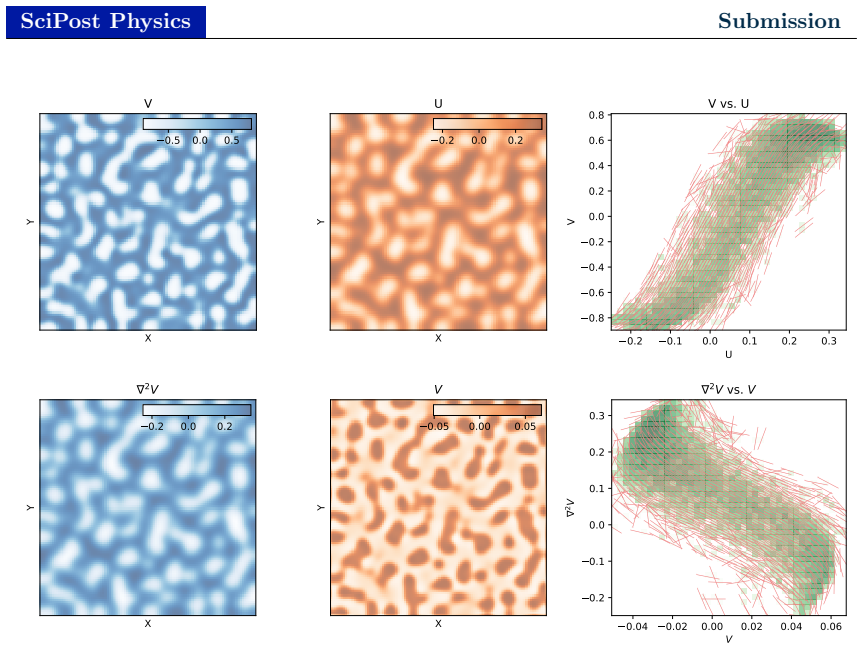
The paper's central claim is that locally correlated variations in spatial data are not noise but a structured signal: when two measured fields are compared in small adjacent regions, their joint changes form a vector field in parameter space. Overlaid on the probability density function, these correlation vectors organize into coherent subregions, and the paper identifies those coherent regions with regimes of different physical behavior. The author asserts that the derived vectors are equivalent to the vector field of a dynamical system on the attracting manifold, and that the adjacent correlation plot is a projected view of that manifold. Under this interpretation, the patterns visible in the plot reflect locally conserved quantities, which appear as straight lines in logarithmic parameter space through a dimensional-analysis argument. The method is demonstrated on simulations of magnetized supersonic turbulence, reaction-diffusion patterns, weather records, and molecular cloud observations.
Load-bearing premise
The method assumes that the average gradient vector in each bin of the parameter plot is a stable and representative description of the local correlations, so that the revealed patterns do not simply follow from the chosen bin size or gradient estimation.
Editorial extensions
If this is right
- A single static snapshot of two fields can be converted into a phase-space vector field, so systems previously compared by a single correlation coefficient can be compared by the geometry of their correlation patterns.
- Regimes with different physics appear as spatially coherent subregions in the adjacent correlation plot, enabling data-driven segregation of a domain before any model is assumed.
- When a locally conserved quantity exists, the corresponding line in the plot can be identified and read as a power-law relation between the two variables in logarithmic space.
- The regularity measure R gives a numeric summary of how much local-law structure a dataset contains and can be used to rank or classify datasets.
- If the vectors are truly equivalent to an attracting-manifold vector field, short-range prediction of the system's behavior from its location in parameter space becomes possible.
Reading between the lines
- Beyond the paper: comparing adjacent correlation plots computed at different bin or patch sizes could serve as a scale-separation diagnostic, locating the range of scales over which the local law is stable.
- Beyond the paper: in time-resolved datasets one can test the forecasting claim directly by checking whether the direction of the correlation vector at a given phase-space location aligns with the observed short-term motion of the data through that space.
- Beyond the paper: the same construction could be extended to three or more variables by replacing the polarization-style sum with a tensor of gradient correlations, which would feed parameter estimation for the governing equations.
Editorial analysis
A structured set of objections, weighed in public.
Referee Report
Summary. The paper introduces Adjacent Correlation Analysis (ACA), a method for extracting local correlations between pairs of spatially distributed fields. For every pixel/voxel, spatial gradients of the two quantities are computed, then these gradient vectors are collected into bins of the joint probability density function and summed as spin-2 objects using a Stokes-parameter construction. The result is an unoriented correlation angle and a degree of coherence p for each bin, plus a scalar regularity measure R. The method is demonstrated on simulations of magnetized turbulence, Turing patterns, NOAA climate data, and molecular cloud observations. The authors interpret the resulting correlation-vector maps as revealing locally conserved quantities and claim that the correlation vectors are equivalent to the vector field of a dynamical system on an attracting manifold, with consequences for classification, prediction, parameter fitting, and forecasting.
Significance. If the central equivalence claim held, ACA would be a valuable and inexpensive tool: a way to turn static spatial snapshots into phase-space vector fields and a regularity measure for classifying datasets. The paper is also commendable for shipping an open-source implementation and for testing the procedure on several genuinely different datasets. However, the construction in Eq. (3) and Appendix A produces a nematic (headless) field, not an oriented first-order vector field, and no derivation or validation connects spatial gradients to time evolution. The descriptive visualization use is plausible and potentially useful, but the predictive and forecasting claims are not supported by the mathematics presented.
major comments (3)
- [Abstract; §5.1; Eq. (3); Appendix A] The headline claim that the ACA correlation vectors are 'equivalent to the vector field in dynamical systems on the attracting manifold' is not supported by the mathematical construction. In Eq. (3), individual gradient vectors are summed as spin-2 objects via the Stokes construction in Appendix A, so opposite vectors cancel and only an orientation modulo 180° survives. A dynamical vector field is an oriented, first-order object whose direction is essential for evolution; the spatial gradient pair (∂p_m/∂x, ∂p_n/∂x) carries no intrinsic arrow of time, and the paper itself notes the 180° rotational symmetry in §5.1. Consequently, the prediction, parameter-fitting, and forecasting implications stated in the abstract and §5.1 do not follow from Eq. (3). Please either remove these claims or support them with an explicit derivation and a validation on a system with known time-ordered dynamics.
- [§3.1; §5.3] The method's reproducibility depends on several parameters that are never specified: the size and shape of the neighborhood in the (p_m, p_n) plane used for binning, the finite-difference stencil used to estimate ∂p_m/∂x and ∂p_n/∂x in Eq. (2), and the weighting factor w_i in Eq. (3). No sensitivity analysis, convergence test, or noise-robustness experiment is reported. Without such checks, the regular patterns that motivate the manifold interpretation in §5.3 (Figs. 3, 4, 8, 9) could be artifacts of the binning or gradient estimation. Please provide a default parameter set, test the method on a synthetic field with a known local relation, and demonstrate that the correlation-vector map is stable under reasonable variations of these parameters.
- [§5.2; Eq. (9)] The derivation of locally conserved quantities contains a typo in Eq. (9): differentiating Eq. (8) should yield α1 d(log q1) + ... + α_i d(log q_i) = 0 (or = d log C = 0), not '= log(C)' with the last term written as d(α_i log q_i). As printed, the equation is dimensionally wrong and cannot support the subsequent claim that locally conserved properties emerge. Please correct the equation and clarify the logical step between the differentiated form and the observed correlations.
minor comments (6)
- [Appendix A, Eq. (12)] The expression for p is missing a square on the (U/I) term; it should read p = sqrt((Q/I)^2 + (U/I)^2).
- [Introduction; §5.1; Fig. 6] The name 'Lorentz' is used throughout; the system in question is the Lorenz system introduced by Lorenz (1963).
- [§4.1] The sentence beginning 'The higher regularity in the logB−logρ indicates...' is garbled and should be rewritten for clarity.
- [§3.1] The code link in the text is blank ('available at .'); please use the GitHub URL given in the Code Availability section.
- [Appendix A] Please define E_x,i and E_y,i explicitly as the components of the gradient vector from Eq. (2); as written, they are introduced as 'measurements' without an explicit connection to the preceding equations.
- [Table 1] The entry 'Bx vs Bys0.21' appears to be a typo; in addition, the regularity values are quoted without uncertainties or a null-model comparison, so the reader cannot judge whether, for example, R=0.25 for the molecular cloud differs meaningfully from chance.
Circularity Check
No significant circularity: the method is a direct, parameter-free descriptor and its interpretive claims are not reductions to fitted inputs or self-cited premises.
full rationale
The core construction is self-contained and non-circular. Equations (2) and (3) define the correlation vector directly from spatial gradients of the input fields, averaged within PDF bins using a spin-2 Stokes sum (Appendix A). No parameter is fitted to any target result, no prediction is generated from a fitted subset of the data, and no load-bearing conclusion is imported from the author's prior work. The only self-citation, [14], is used in Section 4.2 to attach regime labels to an MHD simulation; it is not a premise of the method or of the claimed equivalence. The abstract's statement that the derived vectors are 'equivalent to the vector field in dynamical systems on the attracting manifold' is an interpretive claim, and the paper itself concedes the central difference: 'the vector field has the 180 degrees rotational symmetry' (Section 5.1). That is an overreach or correctness issue, not a circular reduction, because the equivalence is asserted rather than constructed from the definition. Similarly, observing coherent structure in the same data used to build the correlation plot is descriptive pattern reading, not a fitted quantity masquerading as a prediction. No equation reduces to another by definition, and no cited uniqueness or existence theorem is invoked to force the method's choice. Under the quoted-evidence standard, no circular step was found.
Assumptions & free parameters
free parameters (3)
- PDF neighborhood size / bin width
- Gradient estimation stencil
- Weighting factor w_i
assumptions (3)
- domain assumption Spatial gradients of the measured fields are well-defined and capture the local relationship between two quantities.
- domain assumption The studied systems exhibit an attracting manifold with separation of time scales, so that local correlation vectors represent a phase-space vector field.
- domain assumption Local power-law relations (or locally conserved quantities) can be inferred from alignment of the correlation vectors.
Cite this review
Pith. "Pith review of Revealing hidden correlations from complex spatial distributions: Adjacent Correlation Analysis." pith.science (2026). https://pith.science/paper/HVUHLK3F
@misc{pith2026250605759,
  author       = {Pith},
  title        = {Pith review of: Revealing hidden correlations from complex spatial distributions: Adjacent Correlation Analysis},
  year         = {2026},
  howpublished = {\url{https://pith.science/paper/HVUHLK3F}},
  note         = {Machine review of arXiv:2506.05759}
}
read the original abstract
Physics has been transforming our view of nature for centuries. While combining physical knowledge with computational approaches has enabled detailed modeling of physical systems' evolution, understanding the emergence of patterns and structures remains limited. Correlations between quantities are the most reliable approach to describe relationships between different variables. However, for complex patterns, directly searching for correlations is often impractical, as complexity and spatial inhomogeneity can obscure correlations. We discovered that the key is to search for correlations in local regions and developed a new method, adjacent correlation analysis, to extract such correlations and represent them in phase space. When multiple observations are available, a useful way to study a system is to analyze distributions in phase space using the Probability Density Function (PDF). Adjacent correlation analysis evaluates vectors representing local correlations, which can be overlaid on the PDF plot to form the adjacent correlation plot. These correlation vectors often exhibit remarkably regular patterns and may lead to the discovery of new laws. The vectors we derive are equivalent to the vector field in dynamical systems on the attracting manifold. By efficiently representing spatial patterns as correlation vectors in phase space, our approach opens avenues for classification, prediction, parameter fitting, and forecasting.
Figures


Figures from the paper (6 more)



Reference graph
Works this paper leans on
-
[1]
E. N. Lorenz,Deterministic nonperiodic flow, Journal of atmospheric sciences20(2), 130 (1963)
work page 1963
-
[2]
Frisch,Turbulence: The Legacy of AN Kolmogorov, Cambridge University Press (1995)
U. Frisch,Turbulence: The Legacy of AN Kolmogorov, Cambridge University Press (1995)
work page 1995
-
[3]
A. M. Turing,The Chemical Basis of Morphogenesis, Philosophical Trans- actions of the Royal Society of London Series B237(641), 37 (1952), doi:10.1098/rstb.1952.0012
arXiv 1952
-
[4]
M. K. Transtrum, B. B. Machta, K. S. Brown, B. C. Daniels, C. R. Myers and J. P. Sethna,Perspective: Sloppiness and emergent theories in physics, biology, and beyond, The Journal of chemical physics143(1) (2015)
work page 2015
-
[5]
I. G. Kevrekidis and G. Samaey,Equation-Free Multiscale Computation: Algo- rithms and Applications, Annual Review of Physical Chemistry60, 321 (2009), doi:10.1146/annurev.physchem.59.032607.093610
work page Pith review arXiv 2009
-
[6]
U. Maas and S. B. Pope,Simplifying chemical kinetics: intrinsic low-dimensional manifolds in composition space, Combustion and flame88(3-4), 239 (1992)
work page 1992
-
[7]
S. Jain and G. Haller,How to compute invariant manifolds and their reduced dynamics in high-dimensional finite element models, Nonlinear Dynamics107(2), 1417–1450 (2021), doi:10.1007/s11071-021-06957-4
-
[8]
D. C. Collins, A. G. Kritsuk, P. Padoan, H. Li, H. Xu, S. D. Ustyugov and M. L. Norman,The Two States of Star-forming Clouds, Astrophys. J.750(1), 13 (2012), doi:10.1088/0004-637X/750/1/13,1202.2594
arXiv 2012
Show all 18 references
-
[9]
Burkhart, D
B. Burkhart, D. C. Collins and A. Lazarian,Observational Diagnostics of Self- gravitating MHD Turbulence in Giant Molecular Clouds, Astrophys. J.808(1), 48 (2015), doi:10.1088/0004-637X/808/1/48,1505.03855
2015 arXiv
-
[10]
Burkhart, S
B. Burkhart, S. M. Appel, S. Bialy, J. Cho, A. J. Christensen, D. Collins, C. Feder- rath, D. B. Fielding, D. Finkbeiner, A. S. Hill, J. C. Ib´ a˜ nez-Mej ´ ıa, M. R. Krumholz et al.,The Catalogue for Astrophysical Turbulence Simulations (CATS), Astrophys. J.905(1), 14 (2020),...
2020 arXiv
-
[11]
G. G. Stokes,On the composition and resolution of streams of polarized light from different sources, Transactions of the Cambridge Philosophical Society9, 399 (1851). 14 SciPost Physics Submission
-
[12]
Beaumont, A
C. Beaumont, A. Goodman and P. Greenfield,Hackable User Interfaces In Astronomy with Glue, In A. R. Taylor and E. Rosolowsky, eds.,Astronomical Data Analysis Software an Systems XXIV (ADASS XXIV), vol. 495 ofAstronomical Society of the Pacific Conference Series, p. 101 (2015)
2015
-
[13]
Robitaille, C
T. Robitaille, C. Beaumont, P. Qian, M. Borkin and A. Goodman,glueviz v0.13.1: multidimensional data exploration, doi:10.5281/zenodo.1237692 (2017)
2017 doi
- [14]
-
[15]
Skalidis, K
R. Skalidis, K. Tassis and V. Pavlidou,Analytic characterization of sub-Alfv´ enic turbulence energetics, Astron. Astrophys.672, L3 (2023), doi:10.1051/0004- 6361/202346072,2209.14143
2023 arXiv
-
[16]
J. L. Callaham, J. V. Koch, B. W. Brunton, J. N. Kutz and S. L. Brunton,Learning dominant physical processes with data-driven balance models, Nature Communications 12, 1016 (2021), doi:10.1038/s41467-021-21331-z,2001.10019
2021 arXiv
-
[17]
C. J. Dsilva, R. Talmon, C. W. Gear, R. R. Coifman and I. G. Kevrekidis,Data-driven reduction for a class of multiscale fast-slow stochastic dynamical systems, SIAM Journal on Applied Dynamical Systems15(3), 1327 (2016), doi:10.1137/151004896, https://doi.org/10.1137/151004896
2016 doi
-
[18]
S. Kong, H. G. Arce, J. R. Feddersen, J. M. Carpenter, F. Nakamura, Y. Shimajiri, A. Isella, V. Ossenkopf-Okada, A. I. Sargent, ´A. S´ anchez-Monge, S. T. Suri, J. Kauff- mannet al.,The CARMA-NRO Orion Survey, Astrophys. J. Supp. Series236(2), 25 (2018), doi:10.3847/1538-4365/...
2018 arXiv
Reviewed August 7, 2026 · model on record in the stance chip above.
Discussion (0). Sign in to comment.