REVIEW 3 major objections 5 minor 1 cited by
Interpretable Time Series Autoregression for Periodicity Quantification
T0 review · 3 major / 5 minor · reviewed 2026-08-06 · deepseek-v4-flash
Pith's one-line read This paper claims that exact sparse autoregression via mixed-integer optimization extracts the dominant periodic lags from time series and, in temporally and spatially varying forms, scales to millions of real-world mobility and climate…
desk verdict A useful, honest methods paper: exact sparse AR via MIO is not new, but the scaling tricks and the climate-scale maps are, and the two-stage STV-SAR approximation is the soft spot. read the letter →
The pith
A machine-rendered reading of the paper's core claim, the machinery that carries it, and where it could break.
The reading
What carries the argument
The load-bearing object is the binary support vector $z \in \{0,1\}^d$ coupled to the coefficient vector by $0 \le w \le Mz$, so that $w_k$ can be nonzero only when $z_k=1$, together with the global budget $\sum_k z_k \le \tau$. This turns the $\ell_0$ sparsity constraint into a mixed-integer quadratic program that branch-and-bound solvers can solve to proven optimality, which is what distinguishes the method from greedy subspace pursuit. For scalability, the decision variable pruning strategy first screens candidate lags with a fast greedy pass and then solves the reduced MIO, while the two-stage STV-SAR scheme pools all spatial locations into a single global MIO via the trace identity $\sum \|\tilde{x} - Aw\|_2^2 = \operatorname{tr}(ww^\top P) - 2w^\top q + C$ and then solves per-location quadratic programs on the shared support. The selected support set is the model's output: the list of lags that carry the periodicity.
What would settle it
Synthesize a spatial panel in which half the grid cells have a yearly cycle and half are pure noise, run the two-stage STV-SAR pipeline, and compare its global support and per-cell maps against independent per-cell sparse autoregressions; if the aperiodic cells receive nonzero yearly-seasonality coefficients or the yearly lag is missing from the global support, the two-stage approximation is wrong.
Extended reading notes
Core claim
The central claim is that exact sparse autoregression, rather than a dense least-squares fit or a greedy approximation, is the right formulation for periodicity quantification. Concretely, the paper solves $\min_{w,z} \|\tilde{x} - Aw\|_2^2$ subject to $0 \le w \le Mz$, $z \in \{0,1\}^d$, and $\sum_{k=1}^d z_k \le \tau$, where the binary vector $z$ encodes which lags are active and $A$ is the lagged design matrix. A large positive coefficient at lag $k$ is read as periodicity with period $k$, because the model must use that past value to explain the present. The non-stationary extension TV-SAR partitions the series into segments and requires all segments to share the same support set, so that a change in a coefficient means a change in cycle strength, not a change in which cycles exist. The spatiotemporal extension STV-SAR first estimates one global support set from a pooled fit and then estimates per-location coefficients on that support, which is what makes the model tractable for millions of grid cells. The empirical claim is that these models reproduce known cycles, expose structural breaks such as pandemic mobility shifts and Arctic sea surface temperature changes, and flag equatorial Pacific dynamics associated with El Niño.
Load-bearing premise
The load-bearing premise is that one global list of lags, learned by pooling all locations into a single autoregressive fit, is the correct support list for every location; if local cycle structures differ, the two-stage shortcut used for the climate maps can distort the spatial patterns, a bias the authors acknowledge.
Editorial extensions
If this is right
- On hourly NYC ridesharing data with order $d=168$ and sparsity $\tau=4$, TV-SAR selects lags $\{1,24,167,168\}$, identifying local autocorrelation plus daily and weekly cycles; the exact MIO solution achieves a lower objective than non-negative subspace pursuit, which inserts a spurious lag at $k=53$.
- The monthly TV-SAR coefficients show the weekly lag weakening and the daily and local lags strengthening during 2020, then returning to pre-pandemic levels by 2021–2023.
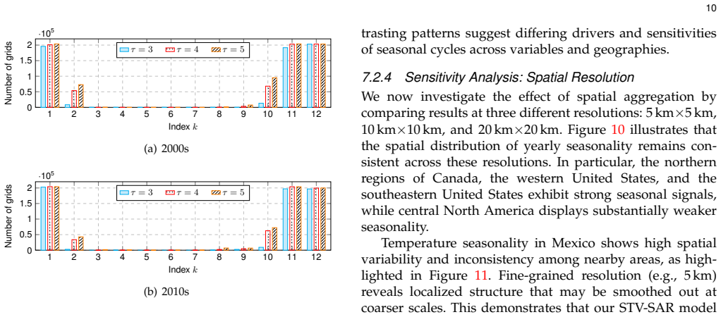
- On the North American Daymet data, STV-SAR maps yearly seasonality with support $\{1,11,12\}$, strong high-latitude signals, an intensification in the 2000s, and consistent patterns at 5, 10, and 20 km resolutions.
- On global sea surface temperatures, the lag-12 coefficient maps show strong seasonality near mid-latitude continents, weaker seasonality in equatorial El Niño zones, and declining Arctic seasonality over recent decades.
- The two-stage STV-SAR pipeline fits over 3.3 million time series at 5 km resolution in under a minute, demonstrating practical scalability.
Reading between the lines
- Beyond the paper's descriptive use, the same selected-lag output could serve as a feature-selection front end for forecasting: if the support is stable across segments, a forecaster could restrict attention to those lags and estimate predictive coefficients without the dense noise.
- The authors concede that the global-support shortcut can bias estimates when local dynamics differ; a natural test is to allow region-specific supports through the paper's sparsely-varying relaxation with a small support-difference budget and compare the resulting seasonality maps on heterogeneous climate zones.
- The method should transfer to other strongly periodic systems, such as energy load, network traffic, or epidemiological counts, where the quantity of interest is precisely which lags carry the cycle and how their weights shift.
- A higher-resolution mobility experiment could test whether the daily lag splits into sub-daily lags when sampling is finer, extending the same support-recovery logic to intra-day periodicities.
Editorial analysis
A structured set of objections, weighed in public.
Referee Report
Summary. The paper proposes a sparse autoregression (SAR) framework with ℓ0-norm sparsity and non-negativity constraints, solved exactly via mixed-integer optimization (MIO). It extends SAR to temporally-varying settings (TV-SAR) with shared support across segments and a decision-variable-pruning acceleration, and to spatiotemporal settings (STV-SAR) with a two-stage scheme that first learns a global support set and then fits per-grid coefficients. Experiments on NYC ridesharing data and on North American/global climate data report interpretable daily, weekly, and yearly periodicities, including shifts attributed to COVID-19 and decadal climate variability. The central claim is that exact sparse AR isolates dominant periodic lags and scales to large real-world spatiotemporal datasets.
Significance. If the claims are fully supported, the framework is a useful interpretable alternative to dense AR and heuristic sparse methods: the MIO formulations are mathematically sound, the selected lags {1,24,168} and {1,11,12} match domain expectations, and the reported scale of millions of time series is impressive. The paper also demonstrates concretely that greedy NNSP can return spurious lags that MIO avoids. The main limitations are the unvalidated two-stage global-support approximation and the absence of uncertainty quantification, which currently weaken the quantitative periodicity claims.
major comments (3)
- [§6.2–6.3, Eq. (13)–(15)] The two-stage global-support approximation is load-bearing for every spatiotemporal map in §7.2–7.3. Eq. (15) forces every per-grid coefficient outside Ω to zero, so an incorrect global support would systematically remove true periodic lags from entire regions rather than merely adding noise. The only validation, Fig. 8, reports aggregate support frequencies for minimum temperature in two decades, but it does not quantify whether the fixed Ω distorts per-grid coefficient estimates, and no analogous check is given for maximum temperature, precipitation, or SST. The conclusion itself concedes that the two-stage scheme 'may lead to estimation bias.' Please add a diagnostic on a sample of grids for each variable/decade comparing the two-stage estimates against local unrestricted or per-grid MIO supports—for example, the fraction of grids where the global support misses the local top lags and the distribution of coefficient differences. Without such a check, the spatial seasonality maps cannot be interpreted as reliable periodicity maps.
- [§7.1.3, §7.2.3, §7.3.2] The empirical periodicity claims are made without uncertainty quantification. The text asserts, for example, that the weekly component 'decreases remarkably' in 2020, that 2019 and 2021–2023 show 'no significant differences,' and that seasonality intensifies in the 2000s, but no standard errors, confidence intervals, or hypothesis tests are reported. The phrase 'no significant differences' in §7.1.3 is therefore unsupported. Please add block-bootstrap or equivalent confidence bands for the reported coefficients and use interval comparisons or tests for the stability/change statements. This is essential because the paper's contribution is periodicity quantification, not merely support-set recovery.
- [§4.3 and §7] The paper claims that MIO gives 'more accurate and reliable periodicity quantification than conventional greedy methods,' but the only baseline is NNSP. There is no comparison with standard periodicity and seasonality tools such as the autocorrelation function, periodogram/spectral analysis, or seasonal-trend decomposition, and no quantitative evaluation on synthetic series with known periods. As a result, the central claim that the selected lags are the 'dominant periodicities' is validated only qualitatively. Please add a benchmark (synthetic ground truth and, ideally, a standard spectral method) or temper the claims about superiority and reliability.
minor comments (5)
- [Eq. (13)] The constraint in Eq. (13) is written as '0 ≤ w ≤ M · z, ∀m, n, γ,' but w is a single global vector; the quantifier should be over the coordinate k ∈ [d].
- [Figure 6 caption] The caption contains a typo ('corresponds to to one month') and the phrase 'accumulated from January to the end of the given month' is unclear; it should specify exactly how the monthly time segments are constructed from the original series.
- [Algorithm 1] Algorithm 1 relies on the NNSP method from [7], but the paper does not provide a self-contained description or pseudocode for NNSP, which is needed to reproduce the DVP experiments.
- [Figure 8] Figure 8 reports support-set frequencies for independent SAR models but does not state which solver was used (NNSP, MIO-DVP, or MIO) or provide any uncertainty quantification; please clarify.
- [Section 5.2] The claim that MIO-DVP 'can be viewed as a backbone-type algorithm' is reasonable, but the sure-screening justification is not established; no screening property (e.g., that the true support is contained in S̃ with high probability) is proven or empirically tested.
Circularity Check
No load-bearing circularity: the sparse AR and two-stage STV-SAR derivations are self-contained, and the authors' self-citations are used as disclosed algorithmic machinery rather than as evidence that forces the periodicity findings.
full rationale
The paper's derivation chain is self-contained. Eq. (5) is the standard big-M mixed-integer reformulation of the l0-constrained least-squares problem in Eq. (4), with binary support variables constructed from the same coefficients being estimated; no target result is inserted. The TV-SAR and STV-SAR objectives in Eqs. (6)-(7) and (9) directly extend that formulation with shared-support constraints and a summed spatiotemporal loss, and the algebra in Eqs. (10)-(14) is a valid trace rearrangement, not an identification assumption. Eq. (15) fixes each local coefficient vector to the globally learned support set Ω; this is an explicit approximation to avoid solving one MIO per grid cell. It is acknowledged in the conclusion that 'the approximation introduced by the two-stage optimization may lead to estimation bias,' which frames it as a statistical/correctness limitation rather than a circularity: the global support is estimated from the data, not defined as the output it is used to explain. The periodicity interpretation rests on the explicit convention in Section 3.2 that 'strong periodicity at lag Δt manifests as a large positive coefficient wΔt'; this is an operational definition of periodicity in terms of AR coefficients, and the optimization does not constrain the selected lags to equal the reported periodicities. The authors' self-citations ([6] for sparsely-varying support MIO, [31] for backbone screening, and [7] for NNSP) are used as disclosed algorithmic building blocks, not as external theorems that force the conclusions. The Fig. 8 support verification further probes the global support against independent per-grid fits, providing a self-contained robustness check. Overall, no equation in the paper reduces to its own output by construction, so circularity is minimal.
Assumptions & free parameters
free parameters (5)
- Sparsity budget tau =
4 (NYC), 3 (climate)
- AR order d =
168 (NYC hourly), 12 (climate monthly)
- Big-M constant M
- DVP pruning threshold tau0 =
5 and 10
- Time segment partition Gamma =
month, decade, 5-year
assumptions (5)
- domain assumption AR residual noise is Gaussian (epsilon_t ~ N(0, sigma^2))
- ad hoc to paper AR coefficients are non-negative
- ad hoc to paper All time segments and spatial cells share the same support set of lags
- ad hoc to paper A single global AR model identifies the correct shared support (STV-SAR stage 1)
- domain assumption MIO solver reaches near-optimal solutions in tractable time
Cite this review
Pith. "Pith review of Interpretable Time Series Autoregression for Periodicity Quantification." pith.science (2026). https://pith.science/paper/I3BK5WAG
@misc{pith2026250622895,
  author       = {Pith},
  title        = {Pith review of: Interpretable Time Series Autoregression for Periodicity Quantification},
  year         = {2026},
  howpublished = {\url{https://pith.science/paper/I3BK5WAG}},
  note         = {Machine review of arXiv:2506.22895}
}
abstract
Time series autoregression (AR) is a classical tool for modeling auto-correlations and periodic structures in real-world systems. We revisit this model from an interpretable machine learning perspective by introducing sparse autoregression (SAR), where $\ell_0$-norm constraints are used to isolate dominant periodicities. We formulate exact mixed-integer optimization (MIO) approaches for both stationary and non-stationary settings and introduce two scalable extensions: a decision variable pruning (DVP) strategy for temporally-varying SAR (TV-SAR), and a two-stage optimization scheme for spatially- and temporally-varying SAR (STV-SAR). These models enable scalable inference on real-world spatiotemporal datasets. We validate our framework on large-scale mobility and climate time series. On NYC ridesharing data, TV-SAR reveals interpretable daily and weekly cycles as well as long-term shifts due to COVID-19. On climate datasets, STV-SAR uncovers the evolving spatial structure of temperature and precipitation seasonality across four decades in North America and detects global sea surface temperature dynamics, including El Ni\~no. Together, our results demonstrate the interpretability, flexibility, and scalability of sparse autoregression for periodicity quantification in complex time series.
Figures


Figures from the paper (11 more)




Forward citations
Cited by 1 Pith paper
-
Data-Driven Discovery of Mobility Periodicity for Understanding Urban Systems
A sparse, non-negative autoregression with coefficients summing to one quantifies weekly periodicity in urban mobility, showing pandemic disruption and recovery across cities and travel modes.
Reference graph
Works this paper leans on
-
[1]
The variability of seasonality,
S. Pezzulli, D. Stephenson, and A. Hannachi, “The variability of seasonality,” Journal of Climate , vol. 18, no. 1, pp. 71–88, 2005
work page 2005
-
[2]
Changes in rainfall seasonality in the tropics,
X. Feng, A. Porporato, and I. Rodriguez-Iturbe, “Changes in rainfall seasonality in the tropics,” Nature Climate Change , vol. 3, no. 9, pp. 811–815, 2013
work page 2013
-
[3]
Seasonality and predictability shape temporal species di- versity,
J. D. Tonkin, M. T. Bogan, N. Bonada, B. Rios-Touma, and D. A. Lytle, “Seasonality and predictability shape temporal species di- versity,” Ecology, vol. 98, no. 5, pp. 1201–1216, 2017
work page 2017
-
[4]
G. E. Box, G. M. Jenkins, G. C. Reinsel, and G. M. Ljung, Time series analysis: forecasting and control . John Wiley & Sons, 2015
2015
-
[5]
J. D. Hamilton, Time series analysis . Princeton university press, 2020
work page 2020
-
[6]
Slowly varying regression under sparsity,
D. Bertsimas, V . Digalakis Jr, M. L. Li, and O. S. Lami, “Slowly varying regression under sparsity,” Operations Research, 2024
work page 2024
-
[7]
Correlating time series with interpretable convolutional kernels,
X. Chen, H. Cai, F. Liu, and J. Zhao, “Correlating time series with interpretable convolutional kernels,” IEEE T ransactions on Knowledge and Data Engineering , 2025
work page 2025
-
[8]
Discovering dynamic patterns from spatiotemporal data with time-varying low-rank autoregression,
X. Chen, C. Zhang, X. Chen, N. Saunier, and L. Sun, “Discovering dynamic patterns from spatiotemporal data with time-varying low-rank autoregression,” IEEE T ransactions on Knowledge and Data Engineering, vol. 36, no. 2, pp. 504–517, 2024
work page 2024
Show all 35 references
-
[9]
J. N. Kutz, S. L. Brunton, B. W. Brunton, and J. L. Proctor, Dynamic mode decomposition: data-driven modeling of complex systems . SIAM, 2016
2016
-
[10]
Time series for macroeconomics and finance,
J. H. Cochrane, “Time series for macroeconomics and finance,” 1997
1997
-
[11]
P . J. Brockwell and R. A. Davis, Time series: theory and methods . Springer science & business media, 1991
1991
-
[12]
A tutorial on estimating time-varying vector autoregressive models,
J. M. Haslbeck, L. F. Bringmann, and L. J. Waldorp, “A tutorial on estimating time-varying vector autoregressive models,” Multivari- ate behavioral research, vol. 56, no. 1, pp. 120–149, 2021
2021
-
[13]
Time- varying autoregression with low-rank tensors,
K. D. Harris, A. Aravkin, R. Rao, and B. W. Brunton, “Time- varying autoregression with low-rank tensors,” SIAM Journal on Applied Dynamical Systems , vol. 20, no. 4, pp. 2335–2358, 2021
2021
-
[14]
Changing dynamics: Time-varying au- toregressive models using generalized additive modeling
L. F. Bringmann, E. L. Hamaker, D. E. Vigo, A. Aubert, D. Bors- boom, and F. Tuerlinckx, “Changing dynamics: Time-varying au- toregressive models using generalized additive modeling.” Psy- chological methods, vol. 22, no. 3, p. 409, 2017. 14
2017
-
[15]
Time varying structural vector autoregressions and monetary policy,
G. E. Primiceri, “Time varying structural vector autoregressions and monetary policy,” The Review of economic studies , vol. 72, no. 3, pp. 821–852, 2005
2005
-
[16]
Autoregressive process modeling via the lasso procedure,
Y. Nardi and A. Rinaldo, “Autoregressive process modeling via the lasso procedure,” Journal of Multivariate Analysis, vol. 102, no. 3, pp. 528–549, 2011
2011
-
[17]
Regression shrinkage and selection via the lasso,
R. Tibshirani, “Regression shrinkage and selection via the lasso,” Journal of the Royal Statistical Society Series B: Statistical Methodology , vol. 58, no. 1, pp. 267–288, 1996
1996
-
[18]
Sparse vector autoregressive modeling,
R. A. Davis, P . Zang, and T. Zheng, “Sparse vector autoregressive modeling,” Journal of Computational and Graphical Statistics , vol. 25, no. 4, pp. 1077–1096, 2016
2016
-
[19]
Discovering governing equations from data by sparse identification of nonlinear dynami- cal systems,
S. L. Brunton, J. L. Proctor, and J. N. Kutz, “Discovering governing equations from data by sparse identification of nonlinear dynami- cal systems,” Proceedings of the national academy of sciences , vol. 113, no. 15, pp. 3932–3937, 2016
2016
-
[20]
Learning sparse nonlinear dynam- ics via mixed-integer optimization,
D. Bertsimas and W. Gurnee, “Learning sparse nonlinear dynam- ics via mixed-integer optimization,” Nonlinear Dynamics, vol. 111, no. 7, pp. 6585–6604, 2023
2023
-
[21]
Okridge: Scalable optimal k-sparse ridge regression,
J. Liu, S. Rosen, C. Zhong, and C. Rudin, “Okridge: Scalable optimal k-sparse ridge regression,” Advances in neural information processing systems, vol. 36, 2024
2024
-
[22]
A sparsity-controlled vector autoregressive model,
E. Carrizosa, A. V . Olivares-Nadal, and P . Ram ´ırez-Cobo, “A sparsity-controlled vector autoregressive model,” Biostatistics, vol. 18, no. 2, pp. 244–259, 2017
2017
-
[23]
Orthogonal matching pursuit: Recursive function approximation with appli- cations to wavelet decomposition,
Y. C. Pati, R. Rezaiifar, and P . S. Krishnaprasad, “Orthogonal matching pursuit: Recursive function approximation with appli- cations to wavelet decomposition,” in Proceedings of 27th Asilomar conference on signals, systems and computers . IEEE, 1993, pp. 40–44
1993
-
[24]
Cosamp: Iterative signal recovery from incomplete and inaccurate samples,
D. Needell and J. A. Tropp, “Cosamp: Iterative signal recovery from incomplete and inaccurate samples,” Applied and computa- tional harmonic analysis , vol. 26, no. 3, pp. 301–321, 2009
2009
-
[25]
Subspace pursuit for compressive sensing signal reconstruction,
W. Dai and O. Milenkovic, “Subspace pursuit for compressive sensing signal reconstruction,” IEEE transactions on Information Theory, vol. 55, no. 5, pp. 2230–2249, 2009
2009
-
[26]
A simple new approach to variable selection in regression, with application to genetic fine mapping,
G. Wang, A. Sarkar, P . Carbonetto, and M. Stephens, “A simple new approach to variable selection in regression, with application to genetic fine mapping,” Journal of the Royal Statistical Society Series B: Statistical Methodology , vol. 82, no. 5, pp. 1273–1300, 2020
2020
-
[27]
Best subset selection via a modern optimization lens,
D. Bertsimas, A. King, and R. Mazumder, “Best subset selection via a modern optimization lens,” 2016
2016
-
[28]
Sparse high-dimensional regres- sion,
D. Bertsimas and B. Van Parys, “Sparse high-dimensional regres- sion,” The Annals of Statistics , vol. 48, no. 1, pp. 300–323, 2020
2020
-
[29]
Sparse regression at scale: Branch-and-bound rooted in first-order optimization,
H. Hazimeh, R. Mazumder, and A. Saab, “Sparse regression at scale: Branch-and-bound rooted in first-order optimization,” Mathematical Programming, vol. 196, no. 1, pp. 347–388, 2022
2022
-
[30]
Rank-one convexification for sparse regression,
A. Atamturk and A. Gomez, “Rank-one convexification for sparse regression,” Journal of Machine Learning Research , vol. 26, no. 35, pp. 1–50, 2025
2025
-
[31]
The backbone method for ultra- high dimensional sparse machine learning,
D. Bertsimas and V . Digalakis Jr, “The backbone method for ultra- high dimensional sparse machine learning,” Machine Learning, vol. 111, no. 6, pp. 2161–2212, 2022
2022
-
[32]
Sure independence screening for ultrahigh dimensional feature space,
J. Fan and J. Lv, “Sure independence screening for ultrahigh dimensional feature space,” Journal of the Royal Statistical Society Series B: Statistical Methodology , vol. 70, no. 5, pp. 849–911, 2008
2008
-
[33]
Safe screening rules for l0-regression from perspective relaxations,
A. Atamturk and A. G ´omez, “Safe screening rules for l0-regression from perspective relaxations,” in International conference on machine learning. PMLR, 2020, pp. 421–430
2020
-
[34]
Daymet: Monthly climate summaries on a 1-km grid for north america, version 4 r1,
M. Thornton, R. Shrestha, Y. Wei, P . Thornton, and S.-C. Kao, “Daymet: Monthly climate summaries on a 1-km grid for north america, version 4 r1,” 2022. [Online]. Available: https://daac.ornl.gov/cgi-bin/dsviewer.pl?ds id=2131 Xinyu Chen is a Postdoctoral Associate at Mas- sac...
2022
-
[2021]
Dingyi Zhuang is a Ph.D
He specializes in continuous optimization, especially in semidefinite programming and ap- plications of optimization in statistics. Dingyi Zhuang is a Ph.D. student in Trans- portation Engineering at MIT Urban Mobility Lab. He received a B.S. degree in Mechanical Engi- neering...
2019
Reviewed August 6, 2026 · model on record in the stance chip above.
Discussion (0). Continue with ORCID to comment.