REVIEW 4 major objections 6 minor 6 references
Comparing Spectrogram Front-Ends for Abnormal Heart-Sound Detection with a Convolutional Neural Network
T0 review · 4 major / 6 minor · reviewed 2026-08-02 · deepseek-v4-flash
Pith's one-line read Choosing how a heart-sound recording is turned into a spectrogram changes how well a fixed neural network finds abnormal heartbeats, with adaptive front-ends beating the plain baseline on the benchmark's official metric.
desk verdict A cleanly run, honestly caveated front-end comparison whose headline ordering is not statistically supported by its own single-seed design. read the letter →
The pith
A machine-rendered reading of the paper's core claim, the machinery that carries it, and where it could break.
The reading
What carries the argument
The key mechanism is the controlled comparison itself: one compact CNN trained three times, once per front-end, with the only difference being the input image. The three front-ends are a vanilla log-mel spectrogram (static decibel compression applied identically to every frequency bin), PCEN (per-channel energy normalization, an automatic gain control that suppresses each channel's slow background and emphasizes locally loud transients such as murmurs), and a multi-resolution log-mel stack (three FFT window sizes — 256, 512, and 1024 samples — stacked as three input channels, trading time resolution against frequency resolution). Because the downstream model and training recipe are identical
What would settle it
Run the same three front-ends over at least five random seeds with the same splits; if PCEN and multi-resolution do not maintain a positive average margin over vanilla log-mel — or if the margin disappears when evaluation is aggregated per recording instead of per clip — the claim that the front-end alone causes the improvement is not supported.
Extended reading notes
Core claim
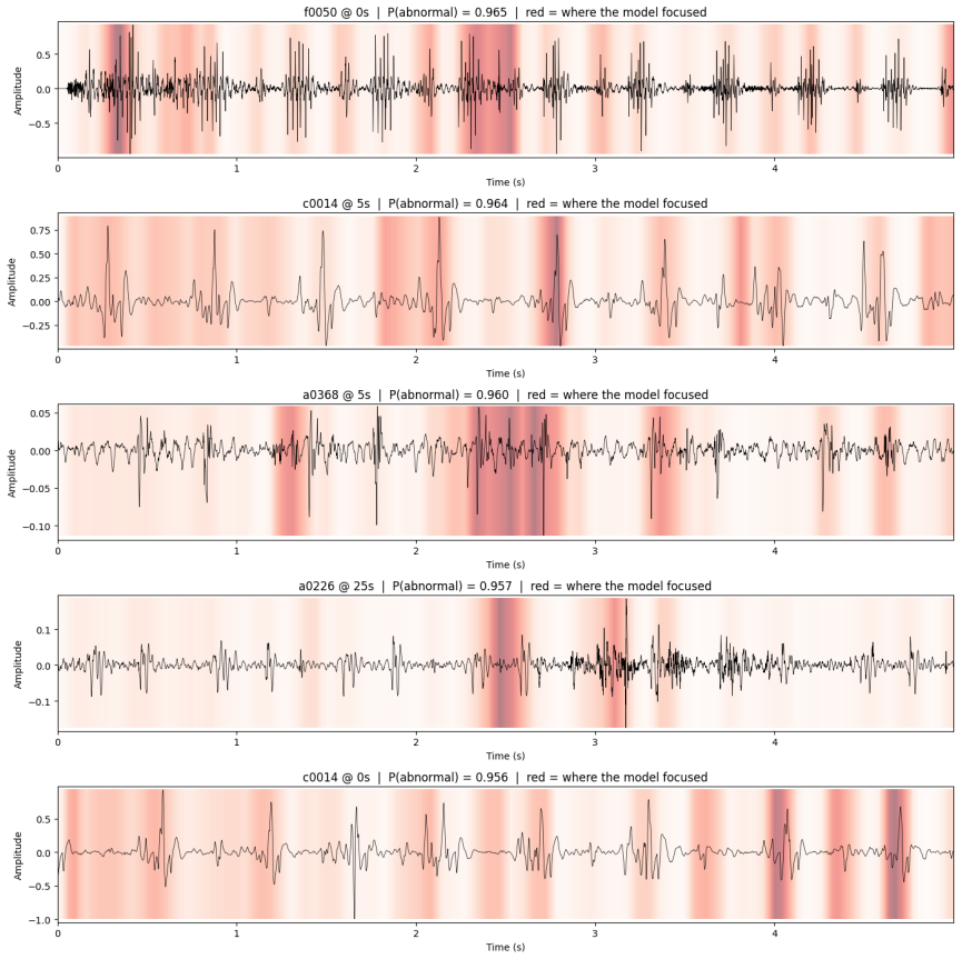
The central claim is that the front-end alone moves the outcome: holding every training condition fixed, PCEN and multi-resolution log-mel both outscore vanilla log-mel on the benchmark's modified-accuracy metric (0.915 and 0.916 versus 0.910), and the gain comes almost entirely from specificity — false alarms on normal clips drop from 197 to 179 and 182 out of 1,984, while sensitivity stays near 0.95. The same pattern is stronger in a smaller two-block network, where the two adaptive front-ends lose only about two points of modified accuracy but the plain baseline loses more than eight. Averaged Grad-CAM maps concentrate on the low-frequency S1/S2 band, with abnormal clips drawing more atte
Load-bearing premise
The ordering of the three front-ends is treated as stable even though the paper reports that rerunning the smaller-network experiment shifts modified accuracy by 0.01–0.02 between seeds, two to four times the 0.005 gaps that separate the front-ends, and test clips from the same recording are counted as independent samples.
Editorial extensions
If this is right
- If the front-end alone shifts the decision boundary, representation design is a viable substitute for architecture or hyperparameter search in low-data audio tasks.
- The false-alarm reduction means an adaptive front-end can lower the cost of follow-up screening without sacrificing abnormal-case detection.
- If the smaller-network result generalizes, an informative representation can let a much smaller model match a larger one, which matters for edge devices and battery-powered stethoscopes.
- Because attention concentrates in the S1/S2 band, the same pipeline may be a foundation for finer-grained classification of specific heart conditions rather than just normal-versus-abnormal.
Reading between the lines
- The authors report that rerunning the smaller architecture changed scores by one to two points between seeds — two to four times the 0.5-point gaps in the main table — so a natural next step is a multi-seed replication; if the average margin does not stay positive, the front-end ordering should be read as a tendency, not a ranking.
- An implication the authors leave implicit is that PCEN's advantage on the smaller network suggests a capacity-for-representation trade: for a fixed accuracy budget, spending computation on the front-end may be cheaper than adding model parameters.
- Because clips from the same recording are correlated, reporting per-recording majority-vote accuracy would clarify whether the apparent 95% sensitivity reflects independent evidence or a handful of recordings.
- The multi-resolution stack's broad attention pattern hints that it may be less sensitive to stethoscope placement and patient-specific timing than single-window front-ends; a cross-dataset test would check that.
Signed reviews
Editorial analysis
A structured set of objections, weighed in public.
Referee Report
Summary. The paper reports a controlled comparison of three spectrogram front-ends — plain log-mel, PCEN, and multi-resolution log-mel — for binary abnormal/normal heart-sound classification on the PhysioNet/CinC 2016 dataset. A fixed compact CNN, optimizer, training schedule, and random seed are used across conditions; only the input representation changes. The central claim is that PCEN and multi-resolution log-mel modestly outperform plain log-mel on the official modified-accuracy metric (0.915 and 0.916 vs 0.910), mainly by reducing false positives on normal clips, and that this advantage persists and even widens when the network is made smaller (§6, §7). Grad-CAM analysis is used to argue that the models attend to low-frequency S1/S2 regions. The paper is written as an independent, non-affiliated project and contains many informal passages and typos.
Significance. If the reported effect were statistically established, the paper would provide a useful empirical data point: for a fixed architecture and training protocol, the spectral front-end can influence specificity without sacrificing abnormal-class sensitivity, and the effect is larger when model capacity is reduced. The design has genuine strengths: a recording-level stratified split (preventing clip-level leakage), a held-out test set chosen by validation F1, identical training conditions across front-ends, and explicit reporting of confusion matrices and the official PhysioNet metric. The authors also honestly flag the run-to-run variance caveat in §9. However, the headline deltas in Table 1 are smaller than the seed-to-seed variation the paper itself reports, which undermines the 'edges out' and 'best-performing' conclusions as currently stated. The clip-level evaluation on correlated clips further overstates the precision of the reported metrics.
major comments (4)
- [§9 and Table 1] The central claim that PCEN and multi-resolution 'edge out' plain log-mel (0.915/0.916 vs 0.910) rests on a single random seed. The paper itself states in §9 that 're-running the smaller-architecture experiment shifted modified accuracy by one to two points between seeds.' That seed-level variation (0.01–0.02) is 2–4 times the size of the Table 1 differences (0.005–0.006), so the observed ordering is one draw from a noisy distribution. The abstract and §6.4 present the ranking as reliable ('consistently beat', 'best-performing'), which overstates the evidence. The authors should either run multiple seeds and report means/variances or substantially temper the claims to 'tendency' as §9 suggests.
- [§3 and Table 1] The test evaluation treats 1,984 clips as independent samples, but these clips come from only 486 recordings and clips from the same recording are strongly correlated. This inflates the effective test size behind sensitivity ≈0.95 and the reported accuracy differences. The paper should use recording-level clustered inference (e.g., cluster bootstrap or aggregating predictions per recording) or at least report confidence intervals that account for this correlation. Without this, the small front-end differences in Table 1 have unknown statistical precision even beyond the seed issue.
- [§6.4 and §7] The statement that multi-resolution 'performs better than the Potes et al first place winner of the PhysioNet 2016 challenge' (§6.4) is not supported by the experiment design. Potes et al. reported on the challenge's hidden test set under the challenge protocol, whereas this paper uses a different split, a different subset of recordings, and a different model-selection rule. Such cross-protocol comparisons are not meaningful and should be removed or heavily qualified.
- [§8 and §9] The Grad-CAM 'low-frequency S1/S2 focus' interpretation is partly by construction: the mel input is band-limited to 20–800 Hz, so the model cannot attend to anything above 800 Hz. Calling the low-frequency attention evidence that 'the network is learning a stable acoustic pattern tied to cardiac function rather than exploiting noise' (§9) is therefore weaker than claimed. To support this, the authors would need to show, for example, that attention localization differs meaningfully from what a model trained on shuffled labels or on a noise-only input would produce, or compare against a baseline with a wider frequency band.
minor comments (6)
- [Throughout] The manuscript contains numerous typos and grammatical errors that impede readability: 'thsi', 'classifer', 'abonral', 'teh', 'purposelfully', 'Mutli-resolution', 'Recoridngs', 'Compariosn', 'indciate', 'heratbeast', 'archiecture', 'arcitecture', etc. A thorough proofread and language edit is needed.
- [Abstract and §1] The abstract's informal tone ('Heart disease kills a lot of people', 'Turns out') is not appropriate for a journal submission. The background section also contains sentence fragments and misspellings that should be corrected.
- [§5 and References] PCEN and Grad-CAM are introduced without citations. The authors should cite the original PCEN paper (Lostanlen et al., 2019) and Grad-CAM (Selvaraju et al., 2017) so readers can verify the implementations.
- [§6.2 and Table 1] The text says 'Both PCEN and the Mutli-resolution improve on the regular vanilla baseline accross all the major metrics, including F1, specificty and the modified Physionet Accruacy'. But Table 1 shows PCEN has sensitivity 0.951 vs vanilla 0.953, i.e., not all metrics improve for both front-ends. Please correct this overstatement.
- [§7] The note from the authors ('I didn't have enoggh compute credits...') is written in first person and breaks the formal register; it should be moved to a limitation paragraph or appendix, and the spelling corrected.
- [§8.1] The Grad-CAM formula uses 'y^c' and 'A^k_{i,j}' without defining 'c' as the class index. A one-sentence definition would improve clarity.
Circularity Check
No central circularity: the front-end comparison is an empirical, held-out evaluation; only the Grad-CAM low-frequency interpretation is partly forced by the band-limited input.
-
self definitional
[§4.1 (front-end definitions) and §8/§9 (Grad-CAM interpretation)]
"All three front-ends begin from a mel-scaled spectrogram, computed with a mel filterbank of Nmel = 64 bins spanning 20–800 Hz ... The network is not really focused on high-frequency sound ... the fact that attention instead concentrates on the low-frequency S1/S2 band is what gives us confidence the learned rule is physiologically grounded."
The mel input is band-limited to 20–800 Hz by construction, so no spectrogram location above 800 Hz exists for Grad-CAM to attend to. The observation that the model 'is not really focused on high-frequency sound' and the claim that low-frequency attention is evidence of physiological grounding are therefore partly artifacts of the input representation, not independent evidence. This does not affect the Table 1 MAcc comparison, which is a direct empirical measurement.
full rationale
The paper's central claim—that PCEN and multi-resolution front-ends slightly outperform vanilla log-mel on the PhysioNet modified accuracy—is an empirical comparison, not a derivation. The same CNN, optimizer, epochs, batch size, and seed are held fixed; the test split is held out; and the reported metrics are computed directly from predictions. There are no fitted parameters renamed as predictions, no uniqueness theorem imported from the authors' prior work, and no load-bearing self-citations (the reference list is entirely external). The only by-construction element is the Grad-CAM interpretation: because every front-end is a mel spectrogram limited to 20–800 Hz, the model cannot attend to frequencies above 800 Hz, so 'attention focuses on low frequencies' is partly guaranteed by the input rather than discovered. That affects the physiological-grounding interpretation in §8–§9, not the quantitative front-end ranking. The paper also honestly flags the single-seed limitation in §9, which is a statistical robustness concern rather than circularity. Overall: no substantive circularity; score 2 for the mild by-construction interpretive point.
Assumptions & free parameters
free parameters (5)
- Spectrogram hyperparameters (n_fft=256, hop=64, n_mels=64, sr=2000, 20–800 Hz band) =
n_fft 256, hop 64, n_mels 64, sr 2000 Hz, mel band 20–800 Hz
- PCEN hyperparameters (s, alpha, delta, r, eps) =
Not reported; librosa defaults assumed
- Multi-resolution window stack nfft ∈ {256, 512, 1024} =
256 / 512 / 1024
- CNN architecture and training hyperparameters =
8/16/32 filters; dropout 0.3; lr 1e-3; 20 epochs; batch 32; class weights 0.63/2.44
- Clip length / resampling (5 s at 2000 Hz) =
5 s (10,000 samples)
assumptions (5)
- domain assumption Every 5-second clip inherits the label of its parent recording; an 'abnormal' recording is assumed abnormal in any clip drawn from it.
- domain assumption The 20–800 Hz mel band contains the discriminative information; frequencies above 800 Hz are safely discarded.
- ad hoc to paper A single run at one fixed random seed gives an estimate whose front-end ordering is meaningful.
- domain assumption Grad-CAM attribution reflects the features the classifier actually relies on, and those features are cardiac physiology rather than recording artifacts.
- domain assumption The transformed spectrograms produced by librosa/torchaudio with unspecified defaults are the canonical PCEN / log-mel / multi-resolution representations.
Cite this review
Pith. "Pith review of Comparing Spectrogram Front-Ends for Abnormal Heart-Sound Detection with a Convolutional Neural Network." pith.science (2026). https://pith.science/paper/I6VWTAHV
@misc{pith2026260716220,
  author       = {Pith},
  title        = {Pith review of: Comparing Spectrogram Front-Ends for Abnormal Heart-Sound Detection with a Convolutional Neural Network},
  year         = {2026},
  howpublished = {\url{https://pith.science/paper/I6VWTAHV}},
  note         = {Machine review of arXiv:2607.16220}
}
read the original abstract
Heart disease kills a lot of people, and one cheap way to catch it early is by listening to heart sounds with a stethoscope, or better yet, just recording them and running them through a model. This project is a binary classification task: take a short clip of someones heartbeat and decide if it sounds normal or abnormal. Instead of trying out a bunch of different models, we kept the CNN the same the whole time and just changed how we turned the raw audio into a picture for it to look at. We tried three ways of doing that: a regular logmel spectrogram, PCEN (which basically normalizes each frequency bin over time), and a multi resolution version that stacks a few different window sizes together. We ran all three on the PhysioNet 2016 heart-sound dataset with the exact same setup but same model, same optimizer, same random seed. Turns out all three do pretty well at catching abnormal cases (sensitivity around 0.95), but PCEN and multi-resolution both edge out the plain logmel on the official PhysioNet accuracy metric (0.915 and 0.916 vs. 0.910). We also ran Grad-CAM to see where the model was actually looking, and it mostly focused on the low frequencies where S1 and S2 heart sounds live, which is a good sign that it learned something real
Figures


Figures from the paper (7 more)



Reference graph
Works this paper leans on
-
[1]
Question 1.Does a vanilla CNN classify heartbeats correctly on its own, or does it require customized front-end adjustments such as PCEN and multi-resolution spectrograms?
-
[2]
Question 2.Trained with the best-performing front-end from Question 1, do different architectures work just as well — i.e., is the best front-end still the best across more than one architecture, or not?
-
[3]
Question 3.What specific part of the heartbeat is the biggest indicator of poor heart health? 3 Dataset The data for this project comes from the PhysioNet/CinC 2016 heart-sound dataset, a publicly available dataset of recorindgs from several independent clinical sources. Each recording is a single-channel .wav audio file accompanied by a reference label o...
arXiv 2016
-
[4]
A., Chorro, F
Liu, C., Springer, D., Li, Q., Moody, B., Juan, R. A., Chorro, F. J., Castells, F., Roig, J. M., Silva, I., Johnson, A. E. W., Syed, Z., Schmidt, S. E., Papadaniil, C. D., Hadjileontiadis, L., Naseri, H., Moukadem, A., Dieterlen, A., Brandt, C., Tang, H., Samieinasab, M., Samieinasab, M. R., Sameni, R., Mark, R. G., & Clifford, G. D. (2016). An open-acces...
2016
-
[5]
Potes, C., Parvaneh, S., Rahman, A., & Conroy, B. (2016). Ensemble of Feature-based and Deep Learning-based Classifiers for Detection of Abnormal Heart Sounds.Computing in Cardiology, 43, 621–624
2016
-
[6]
Rubin, J., Abreu, R., Ganguli, A., Nelaturi, S., Matei, I., & Sricharan, K. (2017). Recognizing Abnormal Heart Sounds Using Deep Learning.arXiv preprintarXiv:1707.04642. 17
arXiv 2017
Reviewed August 2, 2026 · model on record in the stance chip above.
Discussion (0). Continue with ORCID to comment.