REVIEW 1 major objections 5 minor 55 references
Post-training diffusion models on slower, noisier interpolations than their timestep label — MixFlow — closes the train-sampling gap and sets an ImageNet FID of 1.43 without guidance.
Reviewed by Pith at T0; open to challenge. T0 means a machine referee read the full paper against a public rubric. the ladder, T0–T4 →
T0 review · deepseek-v4-flash
2026-08-03 14:44 UTC pith:I7OCA2KT
load-bearing objection MixFlow is a few-line post-training tweak that reliably improves FID across several diffusion/flow models; the exposure-bias explanation is plausible, but the missing label-pairing control keeps me from fully buying the mechanism. the 1 major comments →
MixFlow Training: Alleviating Exposure Bias with Slowed Interpolation Mixture
The pith
A machine-rendered reading of the paper's core claim, the machinery that carries it, and where it could break.
Core claim
The paper claims that exposure bias in diffusion and flow models can be diagnosed and fixed through a single observation: generated noisy data at sampling step t is nearest, in the interpolation geometry, to ground-truth noisy data at a higher-noise timestep m_t ≤ t, which they call the slowed timestep. MixFlow uses this by training u_θ(x_{m_t}, t) toward the velocity u*(x_t, t) of the original timestep, with m_t drawn uniformly from [(1−γ)t, t] and t drawn from Beta(2,1) so the input pairs are sampled evenly. Post-training with this objective consistently improves FID across SiT, REPA, and RAE on ImageNet and on SD3.5 text-to-image, with the largest gains at few-step sampling.
What carries the argument
Slowed interpolation mixture. The input to the velocity network is the interpolation x_{m_t} = β_{m_t} x_0 + α_{m_t} x_1 from a slowed timestep m_t ~ U[(1−γ)t, t], while the conditioning label and the regression target remain those of the training timestep t. The pair-uniform sampling — p(t) ∝ t, i.e., Beta(2,1) — guarantees that all (m_t, t) pairs are visited equally. The mechanism forces the network to map a noisier input to the velocity of a cleaner timestep, the exact correction required when sampling drift makes generated inputs lag behind ground truth.
Load-bearing premise
The load-bearing premise is that regressing the velocity of timestep t from a noisier input x_{m_t} is a valid proxy for the sampling-time mismatch; the paper gives no theory that this objective transfers to sampling, only consistent FID gains on post-trained models.
What would settle it
Train a model with the Beta(2,1) timestep schedule and γ=0 (standard inputs): if it matched MixFlow's FID improvement, the slowed interpolation mixture would not be the cause. Alternatively, measure the prediction error of a MixFlow-trained model on truly generated noisy data at each step t and compare it to the error of the standard model: if the gap does not shrink, the training proxy is not correcting exposure bias.
If this is right
- MixFlow post-training improves gFID on flow matching (SiT), variance-preserving diffusion (SiT-GVP), representation-aligned (REPA), and representation-autoencoder (RAE) models, plus text-to-image generation on SD3.5 at both 40 and 10 sampling steps.
- The benefit increases as the sampling-step budget shrinks: on SiT-B/2, gFID without guidance improves by 2.33 at 250 steps and by 2.58 at 20 steps; on RAE at 256×256, the gain grows from 0.08 at 50 steps to 0.28 at 20 steps.
- With RAE, MixFlow reaches ImageNet 256×256 gFID of 1.43 without guidance and 1.10 with guidance; at 512×512, the scores are 1.55 and 1.10.
- Ablations single out the slowed range as the active ingredient: γ=0 (no mixing) does not improve on the baseline, and including lower-noise interpolations (m_t sampled from [0,1]) hurts performance.
- Initial evidence reported in the paper indicates MixFlow also benefits training SiT from scratch and shortcut models for few-step sampling.
Where Pith is reading between the lines
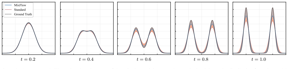
- The mixture coefficient γ could be set from the measured Slow Flow envelope rather than by grid search: RAE's smaller drift motivates its smaller γ=0.4, and the paper's Figure D.1 shows the slowed-timestep envelopes nearly coincide for γ=0.4 and γ=0.8.
- Training with slowed inputs and sampling with shifted timesteps (Time-Shift) attack the same drift from opposite sides; combining them might yield additive gains, since MixFlow makes the network robust to exactly the inputs a shifted sampler produces.
- Annealing γ from large to small over training is a natural curriculum: as MixFlow shrinks the drift (Figure 1b), the optimal slowed range should contract toward γ≈0, possibly improving convergence or final FID.
- The strongest untested implication is for few-step and distillation models, where the sampling trajectory deviates most from ground-truth interpolations; the paper's initial shortcut-model result hints this is where MixFlow could pay off most.
Editorial analysis
A structured set of objections, weighed in public.
Referee Report
Summary. The paper proposes MixFlow, a post-training procedure for diffusion and flow-matching models intended to reduce exposure bias. It first documents a ``Slow Flow'' phenomenon: during sampling, the generated noisy data at timestep t is closest to the ground-truth interpolation at a smaller (higher-noise) slowed timestep m_t ≤ t. MixFlow then trains the prediction network by sampling t ~ Beta(2,1), sampling m_t ~ U[(1−γ)t, t], and optimizing the loss ||u_θ(x_{m_t}, t) − u*(x_t, t)||², i.e., feeding a slowed interpolation while conditioning on the original timestep t and targeting the velocity of x_t. The claimed result is consistent FID improvement across SiT, REPA, RAE, and SD3.5, with new state-of-the-art gFID numbers for RAE on ImageNet (1.43 without guidance, 1.10 with guidance at 256×256). The paper includes several controls: standard post-training (Table 2), a γ=0 control that evaluates Beta(2,1) reweighting alone (Table C.3), and ablation of the m_t sampling range (Table 1, Figure 4).
Significance. If the mechanism is as claimed, the contribution is practically significant: a few lines of code, no sampling-time change, and consistent gains across model families and sampling budgets. The empirical breadth is a real strength, as are the controls ruling out the most obvious confounds: Table 2 shows extra standard post-training does not help, and the γ=0 row in Table C.3 shows Beta(2,1) timestep reweighting alone is not the source of the gain. The method also transfers to representation-aligned models (REPA, RAE) and to text-to-image generation. The main weakness is that the central explanatory mechanism — mixing slowed interpolations while conditioning on the nominal timestep — is not isolated from the simpler possibility that any training on noisier inputs is beneficial. Because the matched-label control is a single ablation, the empirical method is likely salvageable, but the paper as written claims more than the experiments establish.
major comments (1)
- [§4, Eq. (9), Algorithm 1, Table 1] The paper never ablates the conditioning label, so the core mechanism is not isolated. Relative to standard flow matching, MixFlow changes two things: the marginal input distribution (x_mt instead of x_t) and the pairing of the input noise level with the time conditioning t. For the linear interpolant used in the main SiT/flow experiments, u*(x_t,t)=x1−x0 is independent of t, so the target in Eq. (9) is identical to the standard flow-matching target at m_t; the only substantive difference is the time embedding. A matched-label control — sample t and m_t exactly as in MixFlow, but train ||u_θ(x_mt,m_t) − u*(x_mt,m_t)||² — shares the same input marginal and removes the cross-pairing. If this control reaches gFID near MixFlow's 15.64, the improvement is attributable to input-distribution reweighting rather than to the proposed ``slowed interpolation mixture'' exposure-bias mechanism; if it
minor comments (5)
- [§5.1 / Table C.3] The main text says the γ=0 result is ``not shown,'' but it appears in Appendix Table C.3. Since this row is exactly the Beta(2,1)-alone control, it is worth displaying in the main text rather than deferring to the appendix.
- [§5.2 / Table 5 (RAE)] For RAE, the Inception Score decreases after MixFlow in both the guided and unguided settings (e.g., 242.9→239.8 without guidance, 262.6→259.7 with guidance). The text says ``the overall performance gets improved except that the IS scores are a little worse,'' but this trade-off deserves a sentence explaining whether it is systematic or within noise.
- [Appendix G / Figure H.13] The code snippet is labeled with the RAE convention that t=1 is noise, whereas the main paper defines t=1 as data and t=0 as noise. This convention flip is confusing and should be stated clearly whenever the sample code is discussed.
- [Appendix H] The ``Extensions'' section mentions initial results for from-scratch training and shortcut-model training but gives no numbers or protocol. Either include the results or explicitly mark them as preliminary future work, otherwise readers cannot assess the claim.
- [Tables 8 and 9] The SOTA tables list post-training epochs (e.g., MixFlow+RAE 200) next to baselines trained for 800–1400 epochs. Since MixFlow starts from an already-trained checkpoint, the total compute differs. A footnote stating the additional post-training compute would make the comparison easier to interpret.
Circularity Check
No circular derivation; Eq. (9) is a non-tautological training loss and improvements are measured on held-out FID.
full rationale
The load-bearing step is the MixFlow loss in Eq. (9): E_{t,x0,x1,mt}[||u_theta(x_mt,t)-u*(x_t,t)||^2]. This is explicitly different from the standard loss in Eq. (4): the input interpolation is x_mt (a slowed timestep) while the label remains t and the target is u*(x_t,t). Nothing in the loss is set equal to the reported metric: FID/gFID is computed from generated samples of a post-trained model, so the gains (15.64 vs 17.97 for SiT-B; 1.43/1.10 for RAE) are not enforced by construction. The Slow Flow observation is an empirical measurement (Fig. 1, Appendix A, Eq. 12), not a definition of the training loss, and it only motivates the mixture range M_t=[(1-gamma)t,t]. The Beta(2,1) training-timestep distribution is derived from the stated uniformity desideratum p(m_t,t)=const, which is a design choice; the gamma=0 ablation in Table C.3 (18.00/4.48 vs 17.97/4.46) shows the reweighting alone is not responsible for the gain. The paper contains no invoked uniqueness theorem, and the only overlapping-author citations (e.g., [53] in related work) are not load-bearing for the central claim. The absence of a matched-label control (x_mt paired with label m_t) is a legitimate experimental confound for isolating the cross-pairing mechanism, but a missing baseline is not a circular equation; per the review rules, this is a correctness/ablation concern rather than circularity. No step in the derivation reduces to its own input.
Axiom & Free-Parameter Ledger
free parameters (1)
- mixture range coefficient γ =
0.8 (SiT/REPA), 0.4 (RAE); γ=1.0 in the main formulation
axioms (4)
- domain assumption Slow Flow phenomenon: the ground-truth interpolation nearest to generated noisy data at sampling step t lies at a higher-noise timestep m_t ≤ t, and the spread grows roughly linearly with t.
- domain assumption Training on mismatched input/label pairs (x_{m_t}, t) is beneficial: the loss in Eq. (9) with target u*(x_t,t) transfers to better sampling.
- ad hoc to paper Uniform coverage of (m_t,t) pairs is desirable, yielding p(t)=Beta(2,1).
- domain assumption Exposure-bias lag can be measured by L2 projection along the straight interpolation (Eq. 12).
read the original abstract
This paper studies the training-testing discrepancy (a.k.a. exposure bias) problem for improving the diffusion models. During training, the input of a prediction network at one training timestep is the corresponding ground-truth noisy data that is an interpolation of the noise and the data, and during testing, the input is the generated noisy data. We present a novel training approach, named MixFlow, for improving the performance. Our approach is motivated by the Slow Flow phenomenon: the ground-truth interpolation that is the nearest to the generated noisy data at a given sampling timestep is observed to correspond to a higher-noise timestep (termed slowed timestep), i.e., the corresponding ground-truth timestep is slower than the sampling timestep. MixFlow leverages the interpolations at the slowed timesteps, named slowed interpolation mixture, for post-training the prediction network for each training timestep. Experiments over class-conditional image generation (including SiT, REPA, and RAE) and text-to-image generation validate the effectiveness of our approach. Our approach MixFlow over the RAE models achieve strong generation results on ImageNet: 1.43 FID (without guidance) and 1.10 (with guidance) at 256 x 256, and 1.55 FID (without guidance) and 1.10 (with guidance) at 512 x 512.
Figures




Reference graph
Works this paper leans on
-
[1]
Imagenet: A large-scale hierarchical image database
Jia Deng, Wei Dong, Richard Socher, Li-Jia Li, Kai Li, and Li Fei-Fei. Imagenet: A large-scale hierarchical image database. InIEEE Conference on Computer Vision and Pat- tern Recognition (CVPR), 2009. 1, 4
2009
-
[2]
Diffusion models beat gans on image synthesis.Neural Information Process- ing Systems (NeurIPS), 2021
Prafulla Dhariwal and Alexander Nichol. Diffusion models beat gans on image synthesis.Neural Information Process- ing Systems (NeurIPS), 2021. 8
2021
-
[3]
Scaling recti- fied flow transformers for high-resolution image synthesis
Patrick Esser, Sumith Kulal, Andreas Blattmann, Rahim Entezari, Jonas M ¨uller, Harry Saini, Yam Levi, Dominik Lorenz, Axel Sauer, Frederic Boesel, et al. Scaling recti- fied flow transformers for high-resolution image synthesis. InInternational Conference on Machine Learning (ICML),
-
[4]
(b) A bird on theleftof a clock
Patrick Esser, Sumith Kulal, Andreas Blattmann, Rahim 8 (a)Fivesavory pizzas with vibrant red tomato sauce and golden cheese... (b) A bird on theleftof a clock... (c) An oval rug and asquarecoffee table... Figure 5. Example results illustrating the advantages of MixFlow with respect to counting, spatial relationship and object shape. Left: SD 3.5; Middle:...
-
[5]
One step diffusion via shortcut models
Kevin Frans, Danijar Hafner, Sergey Levine, and Pieter Abbeel. One step diffusion via shortcut models. InThe Thirteenth International Conference on Learning Represen- tations, ICLR 2025, Singapore, April 24-28, 2025, 2025. 14
2025
-
[6]
Mdtv2: Masked diffusion transformer is a strong image synthesizer.arXiv preprint arXiv:2303.14389,
Shanghua Gao, Pan Zhou, Ming-Ming Cheng, and Shuicheng Yan. Mdtv2: Masked diffusion transformer is a strong image synthesizer.arXiv preprint arXiv:2303.14389,
-
[7]
Diffit: Diffusion vision transformers for im- age generation
Ali Hatamizadeh, Jiaming Song, Guilin Liu, Jan Kautz, and Arash Vahdat. Diffit: Diffusion vision transformers for im- age generation. InEuropean Conference on Computer Vision (ECCV), 2024. 8
2024
-
[8]
Classifier-free diffusion guidance
Jonathan Ho and Tim Salimans. Classifier-free diffusion guidance. InNeurIPS 2021 Workshop on Deep Generative Models and Downstream Applications, 2021. 2
2021
-
[9]
Denoising dif- fusion probabilistic models.Neural Information Processing Systems (NeurIPS), 2020
Jonathan Ho, Ajay Jain, and Pieter Abbeel. Denoising dif- fusion probabilistic models.Neural Information Processing Systems (NeurIPS), 2020. 2
2020
-
[10]
Simpler diffusion (sid2): 1.5 fid on imagenet512 with pixel-space diffusion
Emiel Hoogeboom, Thomas Mensink, Jonathan Heek, Kay Lamerigts, Ruiqi Gao, and Tim Salimans. Simpler diffusion (sid2): 1.5 fid on imagenet512 with pixel-space diffusion. arXiv preprint arXiv:2410.19324, 2024. 8
Pith/arXiv arXiv 2024
-
[11]
Self forcing: Bridging the train-test gap in autoregressive video diffusion.Neural Information Process- ing Systems (NeurIPS), 2025
Xun Huang, Zhengqi Li, Guande He, Mingyuan Zhou, and Eli Shechtman. Self forcing: Bridging the train-test gap in autoregressive video diffusion.Neural Information Process- ing Systems (NeurIPS), 2025. 1, 2
2025
-
[12]
Fleet, and Ting Chen
Allan Jabri, David J. Fleet, and Ting Chen. Scalable adaptive computation for iterative generation.International Confer- ence on Machine Learning (ICML), 2023. 8
2023
-
[13]
Dengyang Jiang, Mengmeng Wang, Liuzhuozheng Li, Lei Zhang, Haoyu Wang, Wei Wei, Guang Dai, Yanning Zhang, and Jingdong Wang. No other representation component is needed: Diffusion transformers can provide representation guidance by themselves.arXiv preprint arXiv:2505.02831,
-
[14]
Elucidating the design space of diffusion-based generative models.Neural Information Processing Systems (NeurIPS),
Tero Karras, Miika Aittala, Timo Aila, and Samuli Laine. Elucidating the design space of diffusion-based generative models.Neural Information Processing Systems (NeurIPS),
-
[15]
Guiding a diffusion model with a bad version of itself
Tero Karras, Miika Aittala, Tuomas Kynk ¨a¨anniemi, Jaakko Lehtinen, Timo Aila, and Samuli Laine. Guiding a diffusion model with a bad version of itself. InNeural Information Processing Systems (NeurIPS), 2024. 2, 6
2024
-
[16]
Analyzing and improving the training dynamics of diffusion models
Tero Karras, Miika Aittala, Jaakko Lehtinen, Janne Hellsten, Timo Aila, and Samuli Laine. Analyzing and improving the training dynamics of diffusion models. InIEEE Conference on Computer Vision and Pattern Recognition (CVPR), 2024. 8, 16
2024
-
[17]
Variational diffusion models.Neural Information Pro- cessing Systems (NeurIPS), 2021
Diederik Kingma, Tim Salimans, Ben Poole, and Jonathan Ho. Variational diffusion models.Neural Information Pro- cessing Systems (NeurIPS), 2021. 2
2021
-
[18]
Theodoros Kouzelis, Efstathios Karypidis, Ioannis Kakoge- orgiou, Spyros Gidaris, and Nikos Komodakis. Boosting generative image modeling via joint image-feature synthe- sis.arXiv preprint arXiv:2504.16064, 2025. 2
arXiv 2025
-
[19]
Repa-e: Unlocking vae for end-to-end tuning of latent diffusion transformers.IEEE International Conference on Computer Vision (ICCV), 2025
Xingjian Leng, Jaskirat Singh, Yunzhong Hou, Zhenchang Xing, Saining Xie, and Liang Zheng. Repa-e: Unlocking vae for end-to-end tuning of latent diffusion transformers.IEEE International Conference on Computer Vision (ICCV), 2025. 2, 8
2025
-
[20]
Alleviating exposure bias in diffusion mod- els through sampling with shifted time steps.International Conference on Learning Representations (ICLR), 2024
Mingxiao Li, Tingyu Qu, Ruicong Yao, Wei Sun, and Marie- Francine Moens. Alleviating exposure bias in diffusion mod- els through sampling with shifted time steps.International Conference on Learning Representations (ICLR), 2024. 1, 2, 6, 7, 12
2024
-
[21]
Autoregressive image generation without vec- tor quantization.Neural Information Processing Systems (NeurIPS), 2024
Tianhong Li, Yonglong Tian, He Li, Mingyang Deng, and Kaiming He. Autoregressive image generation without vec- tor quantization.Neural Information Processing Systems (NeurIPS), 2024. 8
2024
-
[22]
On error propa- gation of diffusion models
Yangming Li and Mihaela van der Schaar. On error propa- gation of diffusion models. InInternational Conference on Learning Representations (ICLR), 2024. 1
2024
-
[23]
Flow matching for generative modeling
Yaron Lipman, Ricky TQ Chen, Heli Ben-Hamu, Maximil- ian Nickel, and Matthew Le. Flow matching for generative modeling. InInternational Conference on Learning Repre- sentations (ICLR), 2022. 2
2022
-
[24]
Flow straight and fast: Learning to generate and transfer data with rectified flow
Xingchao Liu, Chengyue Gong, et al. Flow straight and fast: Learning to generate and transfer data with rectified flow. InInternational Conference on Learning Representa- tions (ICLR), 2023. 2 9
2023
-
[25]
Instaflow: One step is enough for high-quality diffusion- based text-to-image generation
Xingchao Liu, Xiwen Zhang, Jianzhu Ma, Jian Peng, et al. Instaflow: One step is enough for high-quality diffusion- based text-to-image generation. InInternational Conference on Learning Representations (ICLR), 2023. 2
2023
-
[26]
Sit: Explor- ing flow and diffusion-based generative models with scalable interpolant transformers
Nanye Ma, Mark Goldstein, Michael S Albergo, Nicholas M Boffi, Eric Vanden-Eijnden, and Saining Xie. Sit: Explor- ing flow and diffusion-based generative models with scalable interpolant transformers. InEuropean Conference on Com- puter Vision (ECCV), 2024. 1, 2, 4, 5, 7, 8, 12, 16
2024
-
[27]
Input perturbation reduces exposure bias in diffusion models
Mang Ning, Enver Sangineto, Angelo Porrello, Simone Calderara, and Rita Cucchiara. Input perturbation reduces exposure bias in diffusion models. InInternational Confer- ence on Machine Learning (ICML), 2023. 1, 2, 6, 7, 12
2023
-
[28]
Elucidating the exposure bias in diffusion models.International Conference on Learning Representa- tions (ICLR), 2024
Mang Ning, Mingxiao Li, Jianlin Su, Albert Ali Salah, and Itir Onal Ertugrul. Elucidating the exposure bias in diffusion models.International Conference on Learning Representa- tions (ICLR), 2024. 1, 2, 6, 7, 12
2024
-
[29]
Dinov2: Learning robust visual features without supervision.Transactions on Machine Learning Research (TMLR), 2024
Maxime Oquab, Timoth ´ee Darcet, Th´eo Moutakanni, Huy V V o, Marc Szafraniec, Vasil Khalidov, Pierre Fernandez, Daniel HAZIZA, Francisco Massa, Alaaeldin El-Nouby, et al. Dinov2: Learning robust visual features without supervision.Transactions on Machine Learning Research (TMLR), 2024. 6
2024
-
[30]
Normalizing flows for probabilistic modeling and inference
George Papamakarios, Eric Nalisnick, Danilo Jimenez Rezende, Shakir Mohamed, and Balaji Lakshminarayanan. Normalizing flows for probabilistic modeling and inference. Journal of Machine Learning Research, 2021. 2
2021
-
[31]
Scalable diffusion mod- els with transformers
William Peebles and Saining Xie. Scalable diffusion mod- els with transformers. InIEEE International Conference on Computer Vision (ICCV), 2023. 2, 8, 16
2023
-
[32]
Sequence level training with recurrent neural networks.arXiv preprint arXiv:1511.06732, 2015
Marc’Aurelio Ranzato, Sumit Chopra, Michael Auli, and Wojciech Zaremba. Sequence level training with recurrent neural networks.arXiv preprint arXiv:1511.06732, 2015. 1
Pith/arXiv arXiv 2015
-
[33]
Multi-step denoising scheduled sampling: Towards alleviating exposure bias for diffusion models
Zhiyao Ren, Yibing Zhan, Liang Ding, Gaoang Wang, Chaoyue Wang, Zhongyi Fan, and Dacheng Tao. Multi-step denoising scheduled sampling: Towards alleviating exposure bias for diffusion models. InProceedings of the AAAI Con- ference on Artificial Intelligence, 2024. 1, 2
2024
-
[34]
High-resolution image syn- thesis with latent diffusion models
Robin Rombach, Andreas Blattmann, Dominik Lorenz, Patrick Esser, and Bj¨orn Ommer. High-resolution image syn- thesis with latent diffusion models. InIEEE Conference on Computer Vision and Pattern Recognition (CVPR), 2022. 2
2022
-
[35]
Photorealistic text-to-image diffusion models with deep language understanding.Neural Information Processing Sys- tems (NeurIPS), 2022
Chitwan Saharia, William Chan, Saurabh Saxena, Lala Li, Jay Whang, Emily L Denton, Kamyar Ghasemipour, Raphael Gontijo Lopes, Burcu Karagol Ayan, Tim Salimans, et al. Photorealistic text-to-image diffusion models with deep language understanding.Neural Information Processing Sys- tems (NeurIPS), 2022. 2
2022
-
[36]
Generalization in generation: A closer look at exposure bias.arXiv preprint arXiv:1910.00292, 2019
Florian Schmidt. Generalization in generation: A closer look at exposure bias.arXiv preprint arXiv:1910.00292, 2019. 1
Pith/arXiv arXiv 1910
-
[37]
Denois- ing diffusion implicit models
Jiaming Song, Chenlin Meng, and Stefano Ermon. Denois- ing diffusion implicit models. InInternational Conference on Learning Representations. 2
-
[38]
Selective underfitting in dif- fusion models.arXiv preprint arXiv:2510.01378, 2025
Kiwhan Song, Jaeyeon Kim, Sitan Chen, Yilun Du, Sham Kakade, and Vincent Sitzmann. Selective underfitting in dif- fusion models.arXiv preprint arXiv:2510.01378, 2025. 2
arXiv 2025
-
[39]
Generative modeling by esti- mating gradients of the data distribution.Neural Information Processing Systems (NeurIPS), 2019
Yang Song and Stefano Ermon. Generative modeling by esti- mating gradients of the data distribution.Neural Information Processing Systems (NeurIPS), 2019. 2
2019
-
[40]
Score-based generative modeling through stochastic differential equa- tions
Yang Song, Jascha Sohl-Dickstein, Diederik P Kingma, Ab- hishek Kumar, Stefano Ermon, and Ben Poole. Score-based generative modeling through stochastic differential equa- tions. InInternational Conference on Learning Represen- tations (ICLR), 2021. 2
2021
-
[41]
Contrastive flow match- ing.arXiv preprint arXiv:2506.05350, 2025
George Stoica, Vivek Ramanujan, Xiang Fan, Ali Farhadi, Ranjay Krishna, and Judy Hoffman. Contrastive flow match- ing.arXiv preprint arXiv:2506.05350, 2025. 2
Pith/arXiv arXiv 2025
-
[42]
Ren Sucheng, Yu Qihang, He Ju, Shen Xiaohui, Yuille Alan, and Chen Liang-Chieh. Beyond next-token: Next-x pre- diction for autoregressive visual generation.arXiv preprint arXiv:2502.20388, 2025. 8
Pith/arXiv arXiv 2025
-
[43]
Visual autoregressive modeling: Scalable image gen- eration via next-scale prediction.Neural Information Pro- cessing Systems (NeurIPS), 2024
Keyu Tian, Yi Jiang, Zehuan Yuan, Bingyue Peng, and Liwei Wang. Visual autoregressive modeling: Scalable image gen- eration via next-scale prediction.Neural Information Pro- cessing Systems (NeurIPS), 2024. 8
2024
-
[44]
Runqian Wang and Kaiming He. Diffuse and disperse: Im- age generation with representation regularization.arXiv preprint arXiv:2506.09027, 2025. 2
Pith/arXiv arXiv 2025
-
[45]
Pixnerd: Pixel neural field diffusion.arXiv preprint arXiv:2507.23268, 2025
Shuai Wang, Ziteng Gao, Chenhui Zhu, Weilin Huang, and Limin Wang. Pixnerd: Pixel neural field diffusion.arXiv preprint arXiv:2507.23268, 2025. 8
Pith/arXiv arXiv 2025
-
[46]
Ddt: Decoupled diffusion transformer.arXiv preprint arXiv:2504.05741, 2025
Shuai Wang, Zhi Tian, Weilin Huang, and Limin Wang. Ddt: Decoupled diffusion transformer.arXiv preprint arXiv:2504.05741, 2025. 8
Pith/arXiv arXiv 2025
-
[47]
Representation entanglement for genera- tion: Training diffusion transformers is much easier than you think.Neural Information Processing Systems (NeurIPS),
Ge Wu, Shen Zhang, Ruijing Shi, Shanghua Gao, Zhenyuan Chen, Lei Wang, Zhaowei Chen, Hongcheng Gao, Yao Tang, Jian Yang, et al. Representation entanglement for genera- tion: Training diffusion transformers is much easier than you think.Neural Information Processing Systems (NeurIPS),
-
[48]
Poisson flow generative models.Neural Information Pro- cessing Systems (NeurIPS), 2022
Yilun Xu, Ziming Liu, Max Tegmark, and Tommi Jaakkola. Poisson flow generative models.Neural Information Pro- cessing Systems (NeurIPS), 2022. 2
2022
-
[49]
Reconstruc- tion vs
Jingfeng Yao, Bin Yang, and Xinggang Wang. Reconstruc- tion vs. generation: Taming optimization dilemma in latent diffusion models. InIEEE Conference on Computer Vision and Pattern Recognition (CVPR), 2025. 2, 8
2025
-
[50]
Lijun Yu, Jos ´e Lezama, Nitesh B Gundavarapu, Luca Ver- sari, Kihyuk Sohn, David Minnen, Yong Cheng, Vighnesh Birodkar, Agrim Gupta, Xiuye Gu, et al. Language model beats diffusion–tokenizer is key to visual generation.arXiv preprint arXiv:2310.05737, 2023. 8, 16
Pith/arXiv arXiv 2023
-
[51]
An image is worth 32 tokens for reconstruction and generation.Neural Infor- mation Processing Systems (NeurIPS), 2024
Qihang Yu, Mark Weber, Xueqing Deng, Xiaohui Shen, Daniel Cremers, and Liang-Chieh Chen. An image is worth 32 tokens for reconstruction and generation.Neural Infor- mation Processing Systems (NeurIPS), 2024. 2
2024
-
[52]
Representation alignment for generation: Training diffusion transformers is easier than you think
Sihyun Yu, Sangkyung Kwak, Huiwon Jang, Jongheon Jeong, Jonathan Huang, Jinwoo Shin, and Saining Xie. Representation alignment for generation: Training diffusion transformers is easier than you think. InInternational Con- ference on Learning Representations (ICLR), 2025. 2, 5, 8
2025
-
[53]
Manifold con- 10 straint reduces exposure bias in accelerated diffusion sam- pling.International Conference on Learning Representa- tions (ICLR), 2024
Yao Yuzhe, Chen Jun, Huang Zeyi, Lin Haonan, Wang Mengmeng, Guang Dai, and Wang Jingdong. Manifold con- 10 straint reduces exposure bias in accelerated diffusion sam- pling.International Conference on Learning Representa- tions (ICLR), 2024. 1, 2
2024
-
[54]
Diffusion transformers with representation autoen- coders
Boyang Zheng, Nanye Ma, Shengbang Tong, and Saining Xie. Diffusion transformers with representation autoen- coders. InarXiv preprint arXiv:2510.11690, 2025. 2, 5, 6, 7, 8, 16
Pith/arXiv arXiv 2025
-
[55]
Hongkai Zheng, Weili Nie, Arash Vahdat, and Anima Anandkumar. Fast training of diffusion models with masked transformers.arXiv preprint arXiv:2306.09305, 2023. 8 11 A. Details for Figure 1 Implementation.The ground truth noisy data that is the nearest to the generated noisy data ˆxis the projected data of the generated noisy data along the velocityx 1 −x ...
Pith/arXiv arXiv 2023
discussion (0)
Sign in with ORCID, Apple, or X to comment. Anyone can read and Pith papers without signing in.