REVIEW 2 major objections 4 minor 39 references
A2TTA claims that topology-induced forecasting errors on evolving sensor graphs can be corrected by an expandable, node-conditioned output calibrator attached to a frozen forecaster, with a persistent global state and a disposable local clo
Reviewed by Pith at T0; open to challenge. T0 means a machine referee read the full paper against a public rubric. the ladder, T0–T4 →
T0 review · deepseek-v4-flash
2026-08-03 01:41 UTC pith:IJXSAILQ
load-bearing objection Thorough, unusually honest calibration paper whose central gains hold up; the 'test-time adaptation' label needs a scope warning because each year retrains the backbone and warm-starts on current-year labels. the 2 major comments →
A2TTA: Anchored-and-Agile Test-Time Adaptation for Evolving Traffic Sensor Networks
The pith
A machine-rendered reading of the paper's core claim, the machinery that carries it, and where it could break.
Core claim
The paper's central claim is that the two failure modes of fixed-graph forecasting—topology expansion and multi-scale temporal drift—can be handled without retraining or modifying the deployed forecaster. A2TTA treats the discrepancy between the frozen base forecast and the true traffic values as a node- and horizon-specific calibration error. It appends an expandable node-conditioned FiLM calibrator to the frozen backbone: a shared network that emits per-node, per-horizon scale and shift parameters, so adding new sensors only adds embedding rows while preserving previously learned corrections. Temporal shifts are separated into a persistent global calibrator, updated from causally released
What carries the argument
The load-bearing mechanism is the pair of an expandable node-conditioned FiLM calibrator and an anchored-and-agile state split. FiLM (feature-wise linear modulation) is a small shared network that produces per-node, per-horizon scale and shift corrections conditioned on the base forecast, input history, temporal statistics, and a learnable node embedding; because its parameterization is independent of sensor count, topology growth is absorbed by adding embedding rows. The anchored global state is updated from a bounded pool of causally released labels and kept near its warm-up state via a proximal regularizer, capturing persistent drift, while the agile local clone is copied from the global
Load-bearing premise
The load-bearing premise is that every deployment year supplies a matched backbone checkpoint and a labeled training partition for warm-up; the paper's own warm-up-free control shows that without this labeled start the advantage shrinks, and on TFNSW with Online-AN Avg-MAE rises by 11.4%.
What would settle it
Reproduce A2TTA(OLAN) on TFNSW with the FiLM calibrator initialized as identity and no yearly warm-up—the paper's A.6 control reports Avg-MAE rises by 11.4% relative to the full method; if a broader ten-network replication showed the warm-up-free variant no longer beats the frozen backbone, the claim that A2TTA is a test-time adaptation method rather than a supervised recalibration would be settled against it. A second decisive test: introduce a cohort of sensors that appear only after training with no labels in the current-year partition, and check whether the new-sensor gains (8.8% on PEMS07
If this is right
- With the same frozen backbone checkpoint, attaching A2TTA lowers Avg-MAE by 9.4% on PEMS03, 13.8% on PEMS04, and 29.4% on TFNSW over frozen STAEFormer, and by 33.6% in MAE over Online-AN on TFNSW.
- Gains are especially visible on the metadata-defined new-sensor cohort: MAE falls 8.8% on PEMS07 and 33.7% on TFNSW relative to frozen STAEFormer.
- A2TTA is the best non-foundation method in 119 of 120 per-horizon cells and in 29 of 30 new-sensor panels, and outperforms zero-shot and fine-tuned time-series foundation models in nearly all reported cells.
- The anchored global state plus disposable local clone means transient contexts are corrected without being written back into the persistent model; the clone is used once and discarded, so a single transient event cannot contaminate later forecasts.
- Warm-up matters: removing the three warm-up epochs raises Avg-MAE by up to 11.4% on TFNSW for the Online-AN variant, so the practical benefit depends partly on access to current-year labeled training data.
Where Pith is reading between the lines
- True zero-shot node commissioning—sensors that appear only at test time with no current-year labels—is the obvious stress test the paper does not claim; the warm-up-free results suggest the margin would narrow.
- The anchored/agile split is a transferable recipe: any online system facing multi-scale drift could use a slowly updated state regularized toward initialization plus an ephemeral specialist. A testable variant would spawn the clone only when the context-weight effective sample size drops below the paper's current 0.2·|P| threshold.
- Because the calibrator reads only the base forecast and input features, it could in principle be attached to time-series foundation models themselves; the paper compares against them, not with them, so that combination is untested.
- The output-space diagnostics show the global correction averages 4.40 flow units while the local clone adds 0.90, suggesting the two-stage correction could be tuned further by allocating clone capacity to high-drift windows rather than every window.
Editorial analysis
A structured set of objections, weighed in public.
Referee Report
Summary. The paper proposes A2TTA, a lightweight output-calibration module attached to a frozen traffic-forecasting backbone, targeting sensor networks whose graphs evolve over years. The calibrator uses an expandable node-conditioned FiLM layer and maintains a persistent global state plus a disposable local clone, both updated causally from delayed labels. Evaluations on EvoXXLTraffic and TFNSW across ten networks, two backbones, five seeds, and multiple horizons report consistent MAE/RMSE/MAPE reductions, with A2TTA(STAE) best in 119/120 per-horizon cells and improved new-sensor performance.
Significance. If the results hold as described, the paper demonstrates that a 33K-parameter output calibrator can substantially improve per-year retrained traffic forecasters, and the causal evaluation protocol is careful: leakage-free FIFO pool, matched per-year checkpoints, five paired seeds, sensitivity analyses, and code release. The paper is also unusually transparent about its limitations, including the warm-up dependence and the non-zero-shot nature of new sensors. However, the claimed centrality of online/test-time adaptation is not fully supported by the evidence: the online component contributes little when ablated, while supervised warm-up on current-year training labels accounts for much of the measured gain. The empirical claims are nonetheless internally consistent and reproducible, making the work a useful contribution if the framing is corrected.
major comments (2)
- [Sec. 6.4, Fig. 5; Sec. A.6; Sec. 5.4-5.5] The central claim that A2TTA performs test-time adaptation (Title, Sec. 1) is not fully supported by the evidence because the headline gains are dominated by current-year supervised warm-up rather than the online anchored/agile mechanism. In Sec. 6.4 and Fig. 5, removing all online labels increases median Avg-MAE by only 0.44% (A2TTA(OLAN)) and 0.80% (A2TTA(STAE)). In the ablation (Sec. 6.5, Fig. 6), the 'w/o online TTA' variant nearly matches full A2TTA in most settings. In contrast, Appendix A.6 reports that removing the three warm-up epochs raises Avg-MAE by up to 11.4% (Online-AN on TFNSW), and the warm-up-free control still uses the current-year retrained backbone. Thus the reported 9.4-29.4% reductions over frozen backbones largely reflect supervised calibration on current-year training labels, not online adaptation. Please either add deployment scenarios where online adaptation ma
- [Sec. 4.2, Sec. 6.1; Limitations] The evaluation protocol assumes a matched current-year backbone checkpoint and a labeled training partition for calibrator warm-up each year (Sec. 4.2, Sec. 5.2). No control keeps the backbone fixed from the initial year while adapting only the calibrator. Consequently, the reported improvements conflate annual backbone retraining and current-year supervised calibration with test-time adaptation. The new-sensor results are also not zero-shot because new sensors are present in the current year's training partition (Sec. 4.1, Limitations). Please add a control that uses an initial-year backbone and only the calibrator across years, or explicitly restrict claims to the annually-retrained setting. This is necessary to support the title and abstract framing.
minor comments (4)
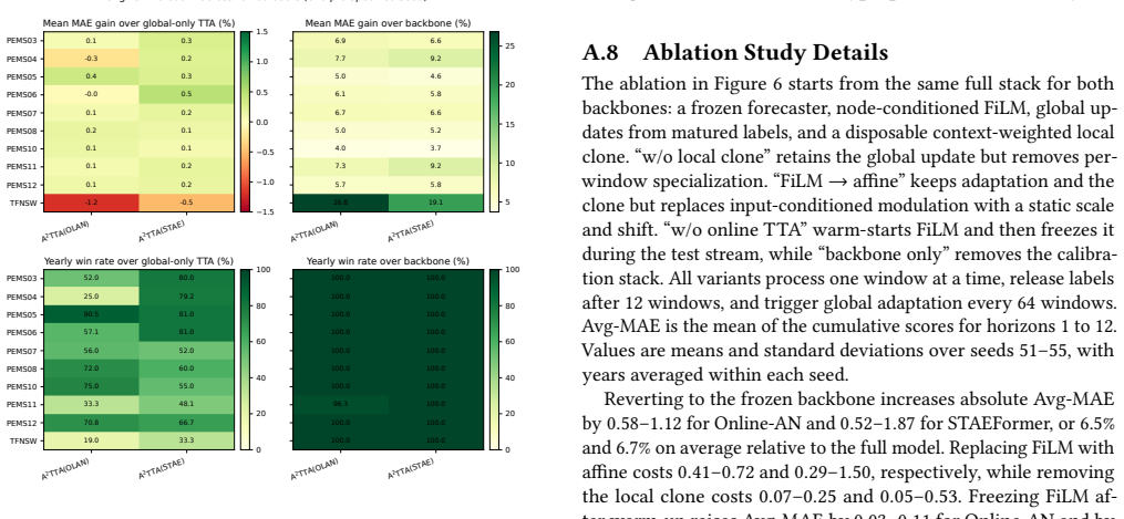
- [A.3.2, Fig. 12] The statement 'A2TTA(STAE) has the lowest error in all 360 combinations' refers to the six plotted methods only; clarify that this holds among the plotted baselines, not all 21 methods.
- [Eq. (11)] The notation for the three weight normalizations is hard to parse; suggest distinct symbols or a small table to separate the raw, clipped, and rescaled weights.
- [Fig. 10 caption] The caption says 'six streams' but the plot shows only four PEMS districts; specify which six data streams are actually included.
- [Sec. 6.8 and A.4] The term 'legacy-batched' is used without definition; clarify how these runs differ from the main one-window chronological protocol, since the figure relies on this distinction.
Circularity Check
No significant circularity: the calibrator is evaluated on out-of-sample windows after delayed label release, and the self-cited benchmark is independent external data.
full rationale
I walked the derivation chain: the FiLM calibrator is initialized to the identity (Eq. 7, zero-initialized output head), warm-started on a chronological training partition, and online updates consume only records released after the full horizon H via the FIFO pool (Eq. 8) and Algorithm 1's causal order. The headline reductions (Sec. 6.3, e.g., 33.6% on TFNSW) are measured on test windows that are not used in those updates, so the reported errors are genuine out-of-sample predictions rather than fitted values renamed as results. The new-sensor cohort is explicitly defined as sensors present in the current year's training partition (Eq. 2, Sec. 4.1), and the Limitations section states it 'should not be interpreted as zero-shot node commissioning,' so no unsupervised prediction is being claimed. The delayed-label sensitivity (Sec. 6.4, Fig. 5) and warm-up-free control (Appendix A.6) quantify the dependence on labeled warm-up rather than concealing it; the dependence is a limitation, not a circular reduction. The only author-overlapping citation is [33] for EvoXXLTraffic, but that is a data benchmark constructed from external PeMS records and the results are corroborated on the external TFNSW network; the central adaptation mechanism does not reduce to that citation. No equation or claim equates an input to its own output by construction.
Axiom & Free-Parameter Ledger
free parameters (6)
- feedback pool capacity M =
512
- global update interval Δ =
64 windows
- adaptation steps K_g, K_l =
3 (local), 3 (global)
- similarity temperature τ, clipping c, ESS floor, ω_tod =
τ=1, c=5, ESS<0.2|P|→uniform, ω_tod=max(S_day/12,1)
- calibrator warm-up epochs =
3
- TTA learning rates =
1e-3 or 3e-3
axioms (5)
- domain assumption Labels eventually arrive for every forecast window (after the H-step horizon)
- domain assumption Current-year labeled training/validation partitions are available for each snapshot, to re-train the yearly backbone checkpoint and warm-start the calibrator
- domain assumption The FiLM parameterization is node-count independent, so new sensors only require adding embedding rows
- domain assumption Yearly graph snapshots with thresholded Gaussian Haversine adjacency (ε=0.1) faithfully represent the evolving network
- standard math Standard deep-learning machinery (shared MLP, AdamW, FiLM conditioning, cosine-similarity retrieval weights) behaves as expected
read the original abstract
Traffic forecasting is important for efficient traffic management and route planning in smart cities. Existing traffic forecasting studies typically assume fixed sensor graphs, overlooking the continuous evolution of real-world traffic networks, e.g., ongoing road network construction and evolving human mobility patterns. These dynamic changes can substantially degrade conventional forecasting models, motivating test-time adaptation (TTA) to efficiently adapt pretrained models during deployment. However, applying TTA to evolving traffic sensor networks remains challenging in two aspects. First, topology expansion introduces new sensors and connections, continuously reshaping the sensor graph. Second, tem- poral shifts vary in time scale and stability, requiring differentiated adaptation to long-term and short-term shifts. In this study, we address these challenges by proposing A2TTA, an Anchored-and-Agile Test-Time Adaptation framework for evolving traffic sensor networks, which transforms topology-induced forecasting errors into an expandable output calibration problem and separates tem- poral adaptation into persistent global correction and agile context-specific specialization. By jointly addressing topology evolution and multi-scale temporal shifts, A2TTA enables efficient and robust adaptation to continuously evolving traffic environments. Extensive experiments on ten real-world traffic networks demonstrate that A2TTA consistently improves forecasting performance across different backbones, datasets, and prediction horizons. Our code is available in https://github.com/lixus7/A2TTA.
Figures



Reference graph
Works this paper leans on
-
[1]
George EP Box, Gwilym M Jenkins, Gregory C Reinsel, and Greta M Ljung. 2015. Time series analysis: forecasting and control. John Wiley & Sons
2015
-
[2]
Pinlong Cai, Yunpeng Wang, Guangquan Lu, Peng Chen, Chuan Ding, and Jian- ping Sun. 2016. A spatiotemporal correlative k-nearest neighbor model for short-term traffic multistep forecasting.Transportation Research Part C: Emerging Technologies62 (2016), 21–34
2016
-
[3]
Chao Chen, Karl Petty, Alexander Skabardonis, Pravin Varaiya, and Zhanfeng Jia. 2001. Freeway performance measurement system: mining loop detector data. Transportation research record1748 (2001), 96–102
2001
-
[4]
Wei Chen and Yuxuan Liang. 2025. Expand and compress: Exploring tuning prin- ciples for continual spatio-temporal graph forecasting. InInternational Conference on Learning Representations, Vol. 2025. 81631–81656
2025
-
[5]
Wei Chen and Yuxuan Liang. 2025. Learning with calibration: Exploring test- time computing of spatio-temporal forecasting.Advances in Neural Information Processing Systems38 (2025), 155895–155929
2025
-
[6]
Xu Chen, Junshan Wang, and Kunqing Xie. 2021. TrafficStream: A Streaming Traf- fic Flow Forecasting Framework Based on Graph Neural Networks and Continual Learning. InProceedings of the Thirtieth International Joint Conference on Artificial Intelligence, IJCAI-21, Zhi-Hua Zhou (Ed.). International Joint Conferences on Artificial Intelligence Organization,...
-
[7]
Zheng Dong, Renhe Jiang, Haotian Gao, Hangchen Liu, Jinliang Deng, Qingsong Wen, and Xuan Song. 2024. Heterogeneity-informed meta-parameter learning for spatiotemporal time series forecasting. InProceedings of the 30th ACM SIGKDD conference on knowledge discovery and data mining. 631–641
2024
-
[8]
Pengxin Guo, Pengrong Jin, Ziyue Li, Lei Bai, and Yu Zhang. 2024. Online Test- Time Adaptation of Spatial-Temporal Traffic Flow Forecasting.arXiv preprint arXiv:2401.04148(2024)
arXiv 2024
-
[9]
Shengnan Guo, Youfang Lin, Ning Feng, Chao Song, and Huaiyu Wan. 2019. Attention based spatial-temporal graph convolutional networks for traffic flow forecasting. InProceedings of the AAAI Conference on Artificial Intelligence, Vol. 33. 922–929
2019
-
[10]
Jiawei Jiang, Chengkai Han, Wayne Xin Zhao, and Jingyuan Wang. 2023. Pdformer: Propagation delay-aware dynamic long-range transformer for traffic flow prediction. InProceedings of the AAAI conference on artificial intelligence, Vol. 37. 4365–4373
2023
-
[11]
Renhe Jiang, Du Yin, Zhaonan Wang, Yizhuo Wang, Jiewen Deng, Hangchen Liu, Zekun Cai, Jinliang Deng, Xuan Song, and Ryosuke Shibasaki. 2021. Dl-traff: Survey and benchmark of deep learning models for urban traffic prediction. In Proceedings of the 30th ACM international conference on information & knowledge management. 4515–4525
2021
-
[12]
Selvaraj Vasantha Kumar. 2017. Traffic flow prediction using Kalman filtering technique.Procedia Engineering187 (2017), 582–587
2017
-
[13]
Yaguang Li, Rose Yu, Cyrus Shahabi, and Yan Liu. 2018. Diffusion Convolutional Recurrent Neural Network: Data-Driven Traffic Forecasting. InInternational Conference on Learning Representations
2018
-
[14]
Aoyu Liu and Yaying Zhang. 2026. A General Spatio-Temporal Backbone with Scalable Contextual Pattern Bank for Urban Continual Forecasting. InThe Four- teenth International Conference on Learning Representations
2026
-
[15]
Hangchen Liu, Zheng Dong, Renhe Jiang, Jiewen Deng, Jinliang Deng, Quan- jun Chen, and Xuan Song. 2023. Spatio-temporal adaptive embedding makes vanilla transformer sota for traffic forecasting. InProceedings of the 32nd ACM international conference on information and knowledge management. 4125–4129
2023
-
[16]
Tengfei Lyu, Weijia Zhang, Jinliang Deng, and Hao Liu. 2025. Autostf: Decoupled neural architecture search for cost-effective automated spatio-temporal forecast- ing. InProceedings of the 31st ACM SIGKDD Conference on Knowledge Discovery and Data Mining V. 1. 985–996
2025
-
[17]
Haoyuan Ma, Mintao Zhou, Xiaodong Ouyang, Du Yin, Renhe Jiang, and Xuan Song. 2022. Forecasting Regional Multimodal Transportation Demand with Graph Neural Networks: An Open Dataset. In2022 IEEE 25th International Conference on Intelligent Transportation Systems (ITSC). IEEE, 3263–3268. doi:10.1109/ITSC55140. 2022.9922512
arXiv 2022
-
[18]
Minbo Ma, Kai Tang, Huan Li, Fei Teng, Dalin Zhang, and Tianrui Li. 2025. Beyond fixed variables: Expanding-variate time series forecasting via flat scheme and spatio-temporal focal learning. InProceedings of the 31st ACM SIGKDD Conference on Knowledge Discovery and Data Mining V. 2. 2054–2065
2025
-
[19]
Florin Schimbinschi, Luis Moreira-Matias, Vinh Xuan Nguyen, and James Bailey
-
[20]
Zezhi Shao, Zhao Zhang, Fei Wang, Wei Wei, and Yongjun Xu. 2022. Spatial- temporal identity: A simple yet effective baseline for multivariate time series forecasting. InProceedings of the 31st ACM international conference on information & knowledge management. 4454–4458
2022
-
[21]
Zezhi Shao, Zhao Zhang, Wei Wei, Fei Wang, Yongjun Xu, Xin Cao, and Chris- tian S Jensen. 2022. Decoupled dynamic spatial-temporal graph neural network for traffic forecasting.Proceedings of the VLDB Endowment15 (2022), 2733–2746. Conference’17, July 2017, Washington, DC, USA Yin et al
2022
-
[22]
Shun-Yao Shih, Fan-Keng Sun, and Hung-yi Lee. 2019. Temporal pattern attention for multivariate time series forecasting.Machine Learning108, 8 (2019), 1421– 1441
2019
-
[23]
Aaron Van Den Oord, Sander Dieleman, Heiga Zen, Karen Simonyan, Oriol Vinyals, Alex Graves, Nal Kalchbrenner, Andrew Senior, Koray Kavukcuoglu, et al
-
[24]
Binwu Wang, Yudong Zhang, Jiahao Shi, Pengkun Wang, Xu Wang, Lei Bai, and Yang Wang. 2023. Knowledge expansion and consolidation for continual traffic prediction with expanding graphs.IEEE Transactions on Intelligent Transportation Systems24, 7 (2023), 7190–7201
2023
-
[25]
Binwu Wang, Yudong Zhang, Xu Wang, Pengkun Wang, Zhengyang Zhou, Lei Bai, and Yang Wang. 2023. Pattern expansion and consolidation on evolving graphs for continual traffic prediction. InProceedings of the 29th ACM SIGKDD Conference on Knowledge Discovery and Data Mining. 2223–2232
2023
-
[26]
Dequan Wang, Evan Shelhamer, Shaoteng Liu, Bruno Olshausen, and Trevor Darrell. 2021. Tent: Fully Test-Time Adaptation by Entropy Minimization. In International Conference on Learning Representations
2021
-
[27]
Billy M Williams and Lester A Hoel. 2003. Modeling and forecasting vehicular traffic flow as a seasonal ARIMA process: Theoretical basis and empirical results. Journal of transportation engineering129, 6 (2003), 664–672
2003
-
[28]
Chun-Hsin Wu, Jan-Ming Ho, and Der-Tsai Lee. 2004. Travel-time prediction with support vector regression.IEEE transactions on intelligent transportation systems5, 4 (2004), 276–281
2004
-
[29]
Zonghan Wu, Shirui Pan, Guodong Long, Jing Jiang, and Chengqi Zhang. 2019. Graph wavenet for deep spatial-temporal graph modeling. InProceedings of the 28th International Joint Conference on Artificial Intelligence. 1907–1913
2019
-
[30]
Mingxing Xu, Wenrui Dai, Chunmiao Liu, Xing Gao, Weiyao Lin, Guo-Jun Qi, and Hongkai Xiong. 2020. Spatial-temporal transformer networks for traffic flow forecasting.arXiv preprint arXiv:2001.02908(2020)
Pith/arXiv arXiv 2020
-
[31]
Du Yin, Jinliang Deng, Shuang Ao, Zechen Li, Hao Xue, Arian Prabowo, Renhe Jiang, Xuan Song, and Flora Salim. 2024. Enhancing Spatio-temporal Quan- tile Forecasting with Curriculum Learning: Lessons Learned. InProceedings of the 32nd ACM International Conference on Advances in Geographic Information Systems. 42–53
2024
-
[32]
Du Yin, Renhe Jiang, Jiewen Deng, Yongkang Li, Yi Xie, Zhongyi Wang, Yifan Zhou, Xuan Song, and Jedi S Shang. 2023. MTMGNN: Multi-time multi-graph neural network for metro passenger flow prediction.GeoInformatica27, 1 (2023), 77–105
2023
-
[33]
Du Yin, Hao Xue, Arian Prabowo, Shuang Ao, and Flora Salim. 2026. From XXLTraffic to EvoXXLTraffic: Scaling Traffic Forecasting to Sensor-Evolving Networks.arXiv preprint arXiv:2605.29768(2026)
Pith/arXiv arXiv 2026
-
[34]
Bing Yu, Haoteng Yin, and Zhanxing Zhu. 2018. Spatio-temporal graph convolu- tional networks: a deep learning framework for traffic forecasting. InProceedings of the 27th International Joint Conference on Artificial Intelligence. 3634–3640
2018
-
[35]
Haoyu Zhang, Hao Miao, Xinke Jiang, Yuchen Fang, and Yifan Zhang. 2025. Strap: Spatio-temporal pattern retrieval for out-of-distribution generalization.Advances in Neural Information Processing Systems38 (2025), 118006–118041
2025
-
[36]
Ling Zhao, Yujiao Song, Chao Zhang, Yu Liu, Pu Wang, Tao Lin, Min Deng, and Haifeng Li. 2019. T-GCN: A temporal graph convolutional network for traffic prediction.IEEE transactions on intelligent transportation systems21, 9 (2019), 3848–3858
2019
-
[37]
w/o local clone
Chuanpan Zheng, Xiaoliang Fan, Cheng Wang, and Jianzhong Qi. 2020. Gman: A graph multi-attention network for traffic prediction. InProceedings of the AAAI conference on artificial intelligence, Vol. 34. 1234–1241. A Appendix A.1 Structural Evolution Details Node counts alone do not characterize this evolution. Figure 11 therefore tracks average node degre...
2020
-
[2016]
Wavenet: A generative model for raw audio.arXiv preprint arXiv:1609.03499 12, 1 (2016)
Pith/arXiv arXiv 2016
-
[2017]
Topology-regularized universal vector autoregression for traffic forecasting in large urban areas.Expert Systems with Applications82 (2017), 301–316
2017
discussion (0)
Sign in with ORCID, Apple, or X to comment. Anyone can read and Pith papers without signing in.