REVIEW 4 major objections 5 minor 6 cited by
A tutorial review argues that the statistical accuracy of diffusion models in simulation-based inference hinges on a few design choices—noise schedule, prediction target, and solver—and recommends specific defaults based on empirical compar
Reviewed by Pith at T0; open to challenge. T0 means a machine referee read the full paper against a public rubric. the ladder, T0–T4 →
Design choices — noise schedule, parameterization, sampler, and model family — measurably change posterior accuracy in diffusion-based SBI; variance-preserving EDM diffusion with adaptive solvers leads on low-dimensional problems, flow matching is competitive on high-dimensional ones.
T0 review reviewed 2026-08-03 challenge →
load-bearing objection Solid tutorial with genuinely useful new comparisons; the MCMC baseline anomaly in Table 4 is the one thing to fix before trusting the high-dimensional rankings. the 4 major comments →
Diffusion Models in Simulation-Based Inference: A Tutorial Review
The pith
A machine-rendered reading of the paper's core claim, the machinery that carries it, and where it could break.
The reading
Core claim
Across the case studies, the paper establishes that posterior accuracy depends strongly, and in a dimension-dependent way, on three interlocking choices: the noise schedule (how signal and noise are mixed over time), the network parameterization (what the network is trained to predict—score, noise, clean target, velocity, or EDM-reconditioned target), and the inference solver (reverse SDE, probability-flow ODE, or few-step consistency). Its headline empirical result is a ranking: variance-preserving EDM schedules with F-parameterization and adaptive SDE solvers are most reliable on low-dimensional benchmarks, flow matching with optimal transport matches them on high-dimensional tasks, and ep
What carries the argument
The time-dependent score, the gradient of the log-density of a noisy state, is the central object; training approximates it by denoising score matching or flow matching, with the noise schedule defining how clean samples and noise are blended. The paper's key identity is that in score space, products of Bayes factors become sums, so a compositional posterior can be assembled from per-observation scores. The design axes are the schedule's log-SNR curve, the weighting over time, the network's prediction target, and the solver.
Load-bearing premise
The empirical rankings rest on reference posteriors that are themselves approximate, such as ABC-SMC ground truths and benchmark references, so if those references are biased—for example by under-resolving a multi-modal posterior—the concluded ordering of methods partly reflects reference artifacts rather than true accuracy.
What would settle it
Compute the same nine-method comparison on a problem with a known analytic posterior or an exact long-run MCMC reference, especially the inverse kinematics problem with multi-modal arm configurations; if the variance-preserving EDM schedule no longer improves classification-based or MMD-based accuracy over cosine or VE schedules, or if epsilon-prediction with Euler does not diverge, the empirical claim fails.
If this is right
- For low-dimensional posterior estimation, users should default to a variance-preserving EDM schedule with an adaptive SDE solver and F- or v-prediction; for high-dimensional problems, flow matching with an adaptive ODE solver is an equally good start.
- Direct epsilon-prediction with Euler sampling should be avoided because it degrades accuracy or diverges, especially in high-dimensional ODE models.
- Compositional score aggregation makes hierarchical models with many groups tractable: a single-subject model reused across subjects can yield global and local posteriors, reducing simulation cost by orders of magnitude.
- Guidance enables changing priors or adding constraints at inference time, but biases the reverse process; a key open question is whether the guided marginals remain statistically valid.
- Consistency models are viable only when inference speed dominates accuracy; in high-dimensional generation they lag diffusion and flow matching.
Where Pith is reading between the lines
- If the dimension-dependent ranking holds beyond the tested cases, one could hypothesize that trajectory straightness and conditioning cost, not family label, predict accuracy; this is testable on problems with intermediate dimensionalities.
- A natural extension is to use the same design-comparison protocol for neural likelihood estimation and joint estimation, where the paper's review suggests the same axes but lacks the head-to-head case study.
- The recommendation set could be sharpened into an adaptive algorithm that selects schedule, parameterization, and sampler based on observed dimension and simulation budget, rather than a fixed default.
- If guidance bias is characterized, inference-time constraint solving could become a general mechanism for scientific models with hard domain constraints, such as positivity or physical bounds.
Editorial analysis
A structured set of objections, weighed in public.
Referee Report
Summary. The paper is a tutorial-review of diffusion models for simulation-based inference (SBI). It develops the score-based formulation, reviews design choices (noise schedules, weighting functions, parameterizations, solvers, model families), describes special uses of scores (guidance, compositional scoring, joint targets, non-Euclidean extensions), and reports four case studies ranging from low-dimensional benchmarks to high-dimensional ODE and random-field models. The empirical protocol is deliberately controlled: architecture and hyperparameters are fixed while only the design choice varies. The paper concludes with prescriptive recommendations, most importantly that practitioners should prefer variance-preserving EDM diffusion models with adaptive SDE solvers, or flow matching with adaptive higher-order ODE solvers, and should avoid direct noise prediction with simple Euler schemes.
Significance. If the empirical findings hold, the paper would be a valuable practical reference: it provides a broad, systematic comparison of design axes, an unusually controlled protocol, public benchmarks, a new GRF benchmark, and explicit reporting of instabilities (e.g., 5% diverged samples for epsilon-prediction, metric limitations in high dimensions). These strengths are real and should be credited. However, the paper's central prescriptive claim is only as strong as its evaluation instruments. The most serious concern is internal: in the high-dimensional case study, the MCMC baseline is ranked last with a very large calibration error, which suggests a problem with the calibration metric or its application rather than with MCMC. Since the high-dimensional rankings feed directly into Section 7, this issue must be resolved before the recommendations can be accepted.
major comments (4)
- [§6.2, Table 4] The MCMC baseline is reported with calibration error 0.427 (MAD 0.217), contraction 1.000, NRMSE 0.124, and ranked 18th of 18. An MCMC sampler targeting the correct Bayesian posterior should be well calibrated; a gold-standard baseline with worst-calibration on a 0–1 scale is a red flag. Because Table 4 is the main evidence for the high-dimensional part of the Section 7 recommendation, please (i) state the exact definition and scaling of the calibration error; (ii) report convergence diagnostics, effective sample sizes, and thinning for the MCMC baseline; (iii) re-rank with an alternative calibration diagnostic (e.g., SBC rank plots, coverage intervals); and (iv) explain why contraction is identically 1.000. If this MCMC result is an artifact, every pairwise ordering in Table 4 is suspect.
- [§6.1 and Figure 4] The C2ST/MMD rankings are computed against reference posteriors: the Lueckmann et al. (2021) “ground-truth” samples and an ABC-SMC reference with acceptance threshold ε_ABC = 0.002 under a 10,000-simulation budget. Both references are approximate; in particular, the inverse-kinematics ABC posterior may under-resolve the multi-modal arm-configuration posterior. No reference uncertainty or alternative reference is reported. Please quantify Monte Carlo error in the reference samples, provide confidence intervals for the C2ST/MMD values, or validate the top-ranked configurations with reference-free diagnostics (e.g., simulation-based calibration, coverage tests). Without this, the claimed ordering (VP-EDM over cosine over VE; SDE over ODE) is partly an assertion about reference quality.
- [§4.1.1, Eq. (18)] Equation (18) states as an identity that ∇_{θ_t} log p(θ_t | y) = ∇_{θ_t} log p(θ_t) + ∇_{θ_t} log p(y | θ_t). For t > 0 this is not an identity unless p(y | θ_t) is defined as the integrated conditional p_t(y | θ_t) = ∫ p(y | θ_0) p(θ_0 | θ_t) dθ_0, which is not the ordinary likelihood. This distinction matters because the guidance framework in Section 4.1 relies on this decomposition. Please state the required approximation explicitly, define the noisy classifier/likelihood term, or derive the exact time-dependent Bayes factorization.
- [§6.2, Table 4 (footnote)] Metrics for the ϵ-prediction models are reported on non-diverged samples only, while 5% diverged during sampling. Conditioning on non-divergence is a form of selection and can bias all metrics; it also understates the practical failure rate of the method. Please report all-sample metrics under a stated convention for diverged samples (e.g., treating them as sampling failures), and give the number of diverged runs for every configuration. This is particularly relevant because the Section 7 recommendation to avoid direct noise prediction is supported by these results.
minor comments (5)
- [§4.2.3, Eq. (37)] Equation (37) appears circular: p(θ^(r)|y,η) ∝ p(θ^(r)|η) p(θ^(r)|y,η). The second factor should presumably be p(y^(r)|θ^(r)), the observation model. Please fix.
- [§7] The global recommendation ‘VP-EDM diffusion with adaptive SDE solver, or flow matching with adaptive ODE solver’ is not fully aligned with Table 4: in the high-dimensional case, the top ranks are flow matching OT/Uniform, then cosine v/F prediction, while EDM VP SDE is ranked 10th. Please stratify the recommendation by dimensionality and explicitly reconcile it with Table 4.
- [Figure 4] The last panel label ‘Cosine -pred.’ is missing the epsilon symbol; it should read ‘Cosine ϵ-pred.’ for consistency with Section 5.4 and Figure 10.
- [§6.1] The text says ABC-SMC was run with ‘a minimum acceptance threshold of ε_ABC = 0.002.’ Please clarify whether this is the final threshold or the minimum over the schedule, and report the number of accepted particles and the effective sample size.
- [§6.2] The sentence ‘For ϵ-prediction, we report the metrics on non-diverged samples’ should also state how many of the 1,000 datasets were affected and whether the divergence rate varied with the solver. This would help readers judge the robustness claim.
Circularity Check
No significant circularity: the review's empirical claims are evaluated against external benchmarks and true simulator parameters, not against outputs derived from its own fitted inputs.
full rationale
The paper's load-bearing empirical claims — that VP-EDM/cosine schedules outperform VE, that adaptive solvers beat simple Euler schemes, and that flow matching with adaptive ODE solvers is competitive — are supported by comparisons with external reference posteriors (Lueckmann et al., 2021 benchmark ground truths), ABC-SMC references, and the true parameters of the Beer et al. (2014) ODE model and the Gaussian random field simulator. These references do not come from the paper's own diffusion models or fitted parameters, so the ranking is not forced by construction. The mathematical equivalences presented in Section 5.4 (Eqs. 57–61) are standard algebraic relations between score, noise, target, velocity, and EDM parameterizations, not circular definitions. Self-citations such as Arruda et al. (2025), BayesFlow 2.0.8 (Radev et al., 2023), and Elsemüller et al. (2025) appear as tools, methods, or background, but the review's central derivations and recommendations do not reduce to these citations; the case studies provide independent evaluation against ground truth. The anomalous MCMC calibration error in Table 4 (0.427 with contraction 1.000 and NRMSE 0.124) is a serious correctness and benchmark-fidelity concern, but it is not an instance of circularity: it does not show that any prediction is equivalent by definition to its input, nor that a fitted parameter was renamed as a prediction. No circular step satisfying the required quote-and-reduction standard is present.
Axiom & Free-Parameter Ledger
free parameters (5)
- EDM schedule hyperparameters (rho, sigma_min, sigma_max) =
7, 0.002, 80
- flow-matching power-law exponent rho =
-0.6
- EDM prediction target variance sigma_target =
1
- error-damping schedule d(t) =
not specified in main text (Arruda et al. 2025)
- mini-batch size M in compositional sampling =
M << R observations
axioms (5)
- standard math Denoising score matching (Vincent 2011), the reverse-SDE drift (Anderson 1982), and the instantaneous change-of-variables formula (Chen et al. 2018) yield valid conditional density estimation.
- standard math The forward process is Gaussian: p(z_t | z_0) = N(alpha_t z_0, sigma_t^2 I), with Gaussian base distribution and Wiener noise.
- domain assumption The simulator defines a joint model p(theta, y) = p(y|theta) p(theta) that can be sampled but not evaluated; the prior can be sampled.
- domain assumption Lueckmann et al. (2021) ground-truth posteriors and the pyABC-SMC reference (epsilon_ABC = 0.002) are accurate measuring instruments for the C2ST/MMD rankings.
- domain assumption Rankings from the four case studies (toy benchmarks, Beer et al. ODE, Gaussian random fields, evidence accumulation model) transfer to the broad class of SBI problems addressed by the Section 7 recommendations.
Cite this review
Pith. "Pith review of Diffusion Models in Simulation-Based Inference: A Tutorial Review." pith.science (2026). https://pith.science/paper/K7RECE7T
@misc{pith2026251220685,
  author       = {Pith},
  title        = {Pith review of: Diffusion Models in Simulation-Based Inference: A Tutorial Review},
  year         = {2026},
  howpublished = {\url{https://pith.science/paper/K7RECE7T}},
  note         = {Machine review of arXiv:2512.20685}
}
read the original abstract
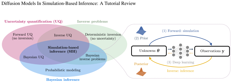
Diffusion models have recently emerged as powerful learners for simulation-based inference (SBI), enabling fast and accurate estimation of latent parameters from simulated and real data. Their score-based formulation offers a flexible way to learn conditional or joint distributions over parameters and observations, thereby providing a versatile solution to various modeling problems. In this tutorial review, we synthesize recent developments on diffusion models for SBI, covering design choices for training, inference, and evaluation. We highlight opportunities created by various concepts such as guidance, score composition, flow matching, consistency models, and joint modeling. Furthermore, we discuss how efficiency and statistical accuracy are affected by noise schedules, parameterizations, and samplers. Finally, we illustrate these concepts with case studies across parameter dimensionalities, simulation budgets, and model types, and outline open questions for future research.
Figures


Forward citations
Cited by 6 Pith papers
-
Hierarchical Bayesian inference with compositional score modeling for stellar streams
Combining three stellar streams and the rotation curve with compositional score modeling yields a posterior for the Milky Way potential—mildly oblate inner halo—but the underlying simulator fails a misspecification test.
-
GenSBI: Generative Methods for Simulation-Based Inference in JAX
GenSBI delivers JAX-native implementations of generative SBI methods with transformer backbones and reports near-ideal calibration scores on standard benchmarks.
-
Rapid and robust simulation-based inference for kilonovae
Simulation-based inference with a Gaussian process emulator trained on ~1300 POSSIS simulations enables rapid, robust kilonova parameter estimation that avoids MCMC biases from likelihood misspecification.
-
Rapid and robust simulation-based inference for kilonovae
A simulation-based inference method with Gaussian process emulators trained on 1300 kilonova simulations recovers parameters accurately and rapidly while avoiding MCMC biases from likelihood misspecification.
-
Overcoming Selection Bias in Statistical Studies With Amortized Bayesian Inference
Embedding selection mechanisms into generative simulators enables amortized Bayesian inference to produce debiased, well-calibrated posteriors without tractable likelihoods.
-
MEmilio -- A high performance Modular EpideMIcs simuLatIOn software for multi-scale and comparative simulations of infectious disease dynamics
MEmilio is a unified, open-source, high-performance epidemic-modeling framework that implements compartmental, metapopulation, agent-based, hybrid, and ML-surrogate models in one C++/Python codebase.
Reference graph
Works this paper leans on
-
[1]
Aitchison, J. (1975). Goodness of prediction fit.Biometrika62.3, pp. 547–554. doi:10.1093/biomet/62.3.547. Anderson, B. D. (1982). Reverse-time diffusion equation models.Stochastic Processes and their Applications12.3, pp. 313–326. doi:10.1016/0304-4149(82)90051-5. Andry, G. (2023). Data assimilation as simulation-based inference. PhD thesis. Université d...
-
[2]
Lake Tahoe, Nevada: Curran Associates Inc., pp
NIPS’13. Lake Tahoe, Nevada: Curran Associates Inc., pp. 2292–2300.https://dl.acm.org/doi/10.5555/2999792.2999868. Daras, G., Chung, H., Lai, C.-H., Mitsufuji, Y ., Ye, J. C., Milanfar, P., Dimakis, A. G., and Delbracio, M. (2024). A survey on diffusion models for inverse problems.arXiv preprint arXiv:2410.00083. doi:10.48550/arXiv.2410.00083. Dasgupta, A...
arXiv 2024
-
[3]
CRC Press. doi:10.1201/9781351075107. Elsemüller, L., Olischläger, H., Schmitt, M., Bürkner, P.-C., Koethe, U., and Radev, S. T. (2024). Sensitivity-Aware Amortized Bayesian Inference.Transactions on Machine Learning Research. https://openreview.net/forum? id=Kxtpa9rvM0. Elsemüller, L., Pratz, V ., Krause, M. von, V oss, A., Bürkner, P.-C., and Radev, S. ...
work page internal anchor Pith review Pith/arXiv arXiv doi:10.48550/arxiv.2502.04949 2024
-
[13]
Montreal, Canada: MIT Press, pp
NIPS’14. Montreal, Canada: MIT Press, pp. 3581–3589. https://dl.acm.org/doi/10.5555/2969033. 2969226. Klir, G. J. (2006). Uncertainty and information: foundations of generalized information theory.Kybernetes35.7/8, pp. 1297–1299. doi:10.1108/03684920610675283. Ko, J. and Geffner, T. (2025). Latent Target Score Matching, with an application to Simulation-B...
-
[17]
Machine learning-enabled velocity model building with uncertainty quantification
Proceedings of Machine Learning Research. PMLR, pp. 16656–16690.https://proceedings.mlr.press/v162/nguyen22e.html. Nichol, A. Q. and Dhariwal, P. (2021). Improved denoising diffusion probabilistic models.International conference on machine learning. PMLR, pp. 8162–8171.https://proceedings.mlr.press/v139/nichol21a. Ohana, R., McCabe, M., Meyer, L. T., More...
work page internal anchor Pith review Pith/arXiv arXiv doi:10.48550/arxiv.2411.06651 2021
-
[19]
Proceedings of Machine Learning Research. PMLR, pp. 28100–28127. https://proceedings.mlr.press/ v202/pooladian23a.html. Radev, S. T., Graw, F., Chen, S., Mutters, N. T., Eichel, V . M., Bärnighausen, T., and Köthe, U. (2021). OutbreakFlow: Model-based Bayesian inference of disease outbreak dynamics with invertible neural networks and its application to th...
arXiv 2021
-
[28]
The Euler–Maruyama adaptive variant followed Fang and Giles (2020), setting the step size proportional to max(1,∥x∥ 2)/max(1,∥v(x)∥
(two-step method with strong order 1.5 for SDEs with additive noise), an adaptive two-step method (Jolicoeur-Martineau et al., 2021), and annealed Langevin dynamics (Song and Ermon, 2019; Song and Ermon, 2020). The Euler–Maruyama adaptive variant followed Fang and Giles (2020), setting the step size proportional to max(1,∥x∥ 2)/max(1,∥v(x)∥
2021
-
[29]
The scheduled variant, uses a fixed step size in the log SNR
with clipping based on minimal/maximal steps. The scheduled variant, uses a fixed step size in the log SNR. The two-step adaptive scheme of Jolicoeur-Martineau et al. (2021) was implemented as an Euler–Heun predictor–corrector: we estimated the local error from the discrepancy between the Euler and Heun updates, compared the normalized error against combi...
2021
-
[32]
Posterior SBC: Simulation-Based Calibration Checking Conditional on Data
doi:10.1007/s11222- 022-10090-6. Säilynoja, T., Schmitt, M., Bürkner, P. -C., and Vehtari, A. (2025). Posterior SBC: Simulation-Based Calibration Checking Conditional on Data.arXiv preprint arXiv:2502.03279. doi:10.48550/arXiv.2502.03279. Salimans, T. and Ho, J. (2022). Progressive distillation for fast sampling of diffusion models.arXiv preprint arXiv:22...
work page internal anchor Pith review Pith/arXiv arXiv doi:10.48550/arxiv.2502.03279 2025
-
[33]
We use a mini-batch size of 3 for the compositional score, and a damping factor of1/number of subjects
and we use the compositional score over all subjects following (Arruda et al., 2025). We use a mini-batch size of 3 for the compositional score, and a damping factor of1/number of subjects. To facilitate training, we represent the starting bias via a Gaussian variable zβ and transform it into a Beta-distributed random variable. Concretely, β= Beta −1(a, b...
2025
-
[35]
478–491.https://dl.acm.org/doi/10.5555/3600270.3600305
Curran Associates, Inc., pp. 478–491.https://dl.acm.org/doi/10.5555/3600270.3600305. Habermann, D., Schmitt, M., Kühmichel, L., Bulling, A., Radev, S. T., and Bürkner, P.-C. (2024). Amortized Bayesian Multilevel Models.arXiv preprint arXiv:2408.13230. doi:10.48550/arXiv.2408.13230. Haitsiukevich, K., Poyraz, O., Marttinen, P., and Ilin, A. (2024). Diffusi...
arXiv 2024
-
[63]
Bansal, A., Chu, H.-M., Schwarzschild, A., Sengupta, S., Goldblum, M., Geiping, J., and Goldstein, T
doi:10.1186/s12918- 017-0433-1. Bansal, A., Chu, H.-M., Schwarzschild, A., Sengupta, S., Goldblum, M., Geiping, J., and Goldstein, T. (2023). Universal guidance for diffusion models.Proceedings of the IEEE/CVF conference on computer vision and pattern recognition, pp. 843–852. doi:10.1109/cvprw59228.2023.00091. Bansal, V ., Chen, T., and Scott, J. G. (202...
arXiv 2023
-
[64]
doi:10.3847/1538-4357/ad8bc3. 42 Diffusion Models In Simulation-Based Inference: A Tutorial Review Nautiyal, M., Hellander, A., and Singh, P. (2025). ConDiSim: Conditional diffusion models for simulation based inference.arXiv preprint arXiv:2505.08403. doi:10.48550/arXiv.2505.08403. Nguyen, K., Nguyen, D., Vu-Le, T.-A., Pham, T., and Ho, N. (2022). Improv...
-
[69]
doi:10.1038/s41540-024-00395-9. Kingma, D. P. (2014). Adam: A method for stochastic optimization.arXiv preprint arXiv:1412.6980. doi:10.48550/arXiv.1412.6980. Kingma, D. P. and Gao, R. (2023). Understanding diffusion objectives as the ELBO with simple data augmentation. Proceedings of the 37th International Conference on Neural Information Processing Syst...
-
[97]
Proceedings of Machine Learning Research. PMLR, pp. 3744–3753.https://proceedings.mlr.press/v97/lee19d.html. 41 Diffusion Models In Simulation-Based Inference: A Tutorial Review Lee, M. D. (2011). How cognitive modeling can benefit from hierarchical Bayesian models.Journal of Mathematical Psychology55.1. Special Issue on Hierarchical Bayesian Models, pp. ...
arXiv 2011
-
[106]
MMD equals zero 48 Diffusion Models In Simulation-Based Inference: A Tutorial Review if and only if the two distributions match in the kernel mean embedding, making it sensitive to discrepancies in mean, covariance, and higher-order moments. Unlike C2ST, MMD does not require training a classifier and exhibits low variance in low-dimensional settings, thou...
2021
-
[108]
Bardenet, R., Doucet, A., and Holmes, C
doi:10.3847/1538-4357/ad9b92. Bardenet, R., Doucet, A., and Holmes, C. (2017). On Markov chain Monte Carlo methods for tall data.Journal of Machine Learning Research18.47, pp. 1–43.http://jmlr.org/papers/v18/15-205.html. Beer, R., Herbst, K., Ignatiadis, N., Kats, I., Adlung, L., Meyer, H., Niopek, D., Christiansen, T., Georgi, F., Kurzawa, N., et al. (20...
arXiv 2017
-
[139]
Proceedings of Machine Learning Research. PMLR, pp. 4629–4640.https://proceedings.mlr. press/v139/izmailov21a.html. Jagvaral, Y ., Mandelbaum, R., and Lanusse, F. (2022). Modeling halo and central galaxy orientations on the SO(3) manifold with score-based generative models.36th Conference on Neural Information Processing Systems. New Orleans, United State...
-
[162]
an exercise in groundwater model calibration and prediction
Proceedings of Machine Learning Research. PMLR, pp. 8867–8887.https://proceedings.mlr.press/v162/hoogeboom22a.html. Houtekamer, P. L. and Zhang, F. (2016). Review of the ensemble Kalman filter for atmospheric data assimilation. Monthly Weather Review144.12, pp. 4489–4532. doi:10.1175/MWR-D-15-0440.1. Huang, D., Bharti, A., Souza, A. H., Acerbi, L., and Ka...
arXiv 2016
-
[202]
Proceedings of Machine Learning Research. PMLR, pp. 11098– 11116.https://proceedings.mlr.press/v202/geffner23a.html. Gelman, A., Carlin, J. B., Stern, H. S., Dunson, D. B., Vehtari, A., and Rubin, D. B. (2013).Bayesian Data Analysis (3rd Edition). Chapman and Hall/CRC. doi:10.1201/b16018. Gelman, A., Carlin, J. B., Stern, H. S., and Rubin, D. B. (1995).Ba...
arXiv 2013
-
[258]
Proceedings of Machine Learning Research. PMLR, pp. 2377–2385. https://proceedings.mlr.press/v258/chen25d.html. Chen, T., ZHANG, R., and Hinton, G. (2023a). Analog Bits: Generating Discrete Data using Diffusion Models with Self-Conditioning.The Eleventh International Conference on Learning Representations. https://openreview. net/forum?id=3itjR9QxFw. 37 D...
-
[1988]
Springer, pp. 455–466. doi:10.1007/978-94-015-7860-8_48. Song, J., Meng, C., and Ermon, S. (2021a). Denoising Diffusion Implicit Models.International Conference on Learning Representations.https://openreview.net/forum?id=St1giarCHLP. Song, Y . and Dhariwal, P. (2024). Improved Techniques for Training Consistency Models.The Twelfth International Conference...
arXiv 2024
-
[2014]
ground-truth
of 0.05 is used for all models. Code to reproduce the experiments is available at github.com/bayesflow-org/diffusion-experiments. EMAAdditionally, we evaluate whether applying an exponential moving average (EMA) to model parameters improves performance. EMA maintains a smoothed version of the network weights ˆψ by updating them as a weighted average of pa...
2024
-
[2017]
A compact multilayer perceptron serves as the core backbone for all models
with an initial value of 5e-4. A compact multilayer perceptron serves as the core backbone for all models. It consists of five fully connected layers with width 256, Mish activations (Misra, 2019), He normal initialization (He et al., 2015), and residual connections (He et al., 2016). Targets and conditions are concatenated together and mapped to a shared...
2019
-
[2020]
(2023), while the residual blocks use a linear FiLM conditioning (Perez et al.,
of dimension 32 similar to Wildberger et al. (2023), while the residual blocks use a linear FiLM conditioning (Perez et al.,
2023
-
[2021]
statistic
with settings as described before in Section A.1.1. As a classifier, we use a sequence of two MLPs with width of 128 and 5-fold cross-validation. 52 Diffusion Models In Simulation-Based Inference: A Tutorial Review We ran all analyses on a computing cluster. The computing cluster used an Intel Xeon Sapphire Rapids CPU with a core clock speed of up to 2.1 ...
2022
-
[2023]
Due to the high dimensions, exploring the parameter space is difficult even for the adaptive parallel tempering algorithm
as overall multi-chain algorithms perform better than single-chain algorithms (Ballnus et al., 2017). Due to the high dimensions, exploring the parameter space is difficult even for the adaptive parallel tempering algorithm. ArchitectureTo obtain a scalar comparison across methods, we rank them by the sum of ECE and NRMSE. For this setting, we combine the...
2017
-
[2024]
https://ml4physicalsciences.github.io/2024/files/ NeurIPS_ML4PS_2024_26.pdf. Foster, J. M., Dos Reis, G., and Strange, C. (2024). High order splitting methods for SDEs satisfying a commutativity condition.SIAM Journal on Numerical Analysis62.1, pp. 500–532. doi:10.1137/23M161077X. Frazier, D. T., Kelly, R., Drovandi, C., and Warne, D. J. (2024). The stati...
-
[2025]
https://ml4physicalsciences.github.io/ 2025/files/NeurIPS_ML4PS_2025_8.pdf. Krause, M. von, Radev, S. T., and V oss, A. (2022). Mental speed is high until age 60 as revealed by analysis of over a million participants.Nature human behaviour6.5, pp. 700–708. doi:10.1038/s41562-021-01282-7. Kruse, J., Ardizzone, L., Rother, C., and Köthe, U. (2021). Benchmar...
-
[3833]
doi:10.3390/electronics14193833. – (2025b). Flow Matching Posterior Estimation for Simulation-based Atmospheric Retrieval of Exoplanets.IEEE Access. doi:10.1109/access.2025.3594751. Osada, G., Shing, M., and Nishide, T. (2024). Local Curvature Smoothing with Stein’s Identity for Efficient Score Matching.The Thirty-eighth Annual Conference on Neural Inform...
arXiv 2025
-
[4304]
doi:10.21105/joss.04304. Schmitt, M., Bürkner, P. -C., Köthe, U., and Radev, S. T. (2023). Detecting model misspecification in amortized Bayesian inference with neural networks.Dagm german conference on pattern recognition. Springer, pp. 541–557. doi:10.1007/978-3-031-54605-1_35. Schmitt, M., Pratz, V ., Köthe, U., Bürkner, P.-C., and Radev, S. T. (2025)....
arXiv 2023
-
[5702]
doi:10.21105/joss.05702. Ratcliff, R., Smith, P. L., Brown, S. D., and McKoon, G. (2016). Diffusion decision model: Current issues and history. Trends in cognitive sciences20.4, pp. 260–281. doi:10.1016/j.tics.2016.01.007. Raymond, V ., Al-Shammari, S., and Göttel, A. (2025). Simulation-based inference for gravitational-waves from intermediate-mass binary...
Pith/arXiv arXiv 2016
This paper was first reviewed by deepseek-v4-flash on August 3, 2026.
discussion (0)
Sign in with ORCID, Apple, or X to comment. Anyone can read and Pith papers without signing in.