REVIEW 4 major objections 4 minor 53 references
Pre-trained LLMs solving HMM next-token prediction do not run Bayesian inference; they learn finite-window, gradient-descent-like approximations described by Soft n-gram statistics.
Reviewed by Pith at T0; open to challenge. T0 means a machine referee read the full paper against a public rubric. the ladder, T0–T4 →
T0 review · deepseek-v4-flash
2026-08-02 10:05 UTC pith:LUTV4YT4
load-bearing objection Good empirical pipeline and a clean small-transformer result, but the headline finite-window claim is not supported by the Soft n-gram probe, which refits weights on the full context. the 4 major comments →
Extracting Algorithms in Pre-trained LLMs: A Case on Hidden Markov Models
The pith
A machine-rendered reading of the paper's core claim, the machinery that carries it, and where it could break.
Core claim
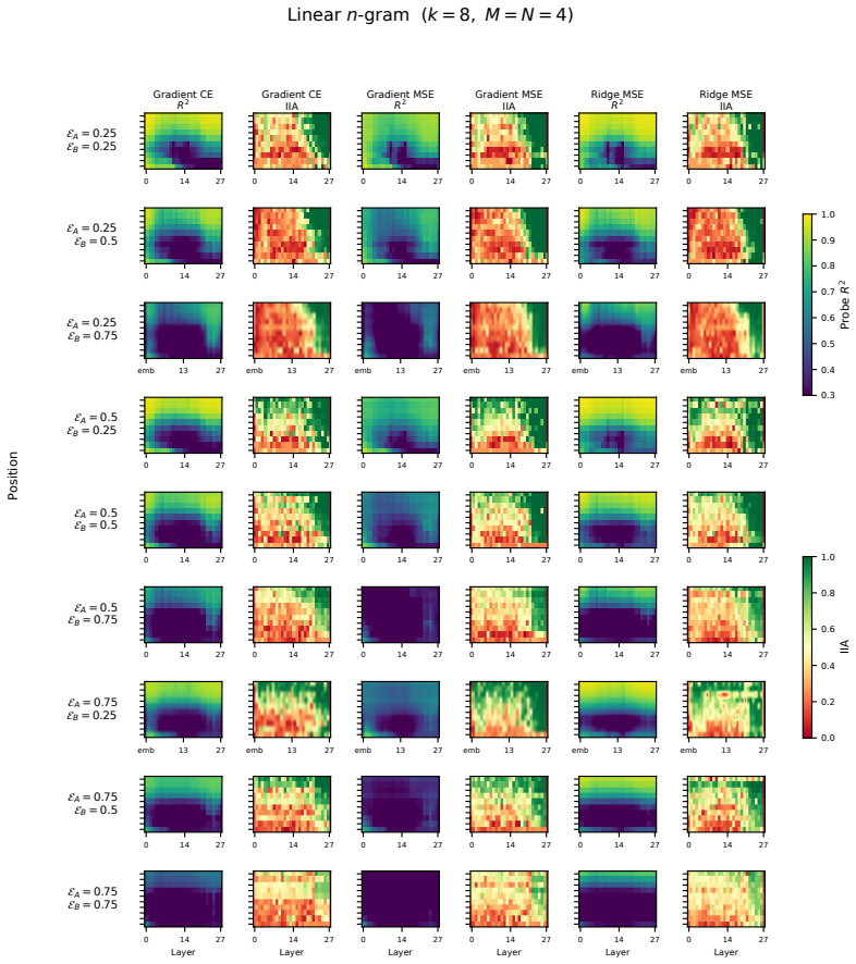
On HMM next-token prediction, pre-trained LLM predictions converge toward the Bayes-optimal oracle as context grows, but the internal algorithm responsible is not belief tracking or spectral filtering. Using PAP, the paper shows low-dimensional linear representations in the residual stream causally drive predictions, and that the Soft n-gram representation—a linearly learned predictor over a finite window of recent observations—is the most causally effective algorithmic state across different HMM regimes. The same probing shows that algorithmic information can be decodable without being causally used: early layers may encode beliefs that downstream computation bypasses. In a small Transforme
What carries the argument
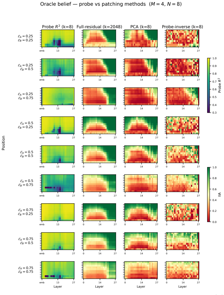
The Principal Activations Probe (PAP) is the central tool: it projects layer-wise residual activations onto their top principal components, fits a ridge regression from those coordinates to candidate algorithmic representations (Oracle belief, Soft n-gram belief/operator, Spectral belief/operator), and then tests causal use with three escalating patches—full residual, PCA-subspace, and probe-inverse. The underlying theoretical identity is Lemma 3.1: the Bayes-optimal next-token distribution is linear in the Kronecker product of the last n one-hot observations, which unifies the n-gram, nonlinear-feature, and spectral constructions and justifies why a finite-window linear predictor can approx
Load-bearing premise
The causal conclusion rests on the assumption that patching the probe's readout directions replaces the algorithm the model uses, rather than overwriting its next-token distribution near the output; since the Soft n-gram belief is itself a next-token distribution, the two can be hard to distinguish.
What would settle it
Construct source/target histories that share the same last n observations but differ in earlier context, so the Soft n-gram belief W_t z_t changes only through the full-context-refit weight W_t; if patching this belief still shifts the LLM output, the causal effect is coming from long-context weights, not the finite-window feature itself.
If this is right
- LLMs can match Bayes-optimal HMM predictions while internally implementing a finite-window, n-gram-like algorithm, so behavioral convergence alone does not reveal the learned mechanism.
- Decodability and causal use must be tested separately: a representation can be present in activations yet not drive predictions.
- The internally recruited representation shifts with HMM regime: richer Soft n-gram tracking is used when belief integration matters, while bigram-like statistics suffice when emissions are nearly deterministic.
- Distinct computational stages localize to different layers, with early layers often encoding information that later layers bypass.
- A small Transformer trained on a fixed HMM learns a finite-window predictor almost exactly, suggesting this algorithm class is a natural inductive outcome of the architecture.
Where Pith is reading between the lines
- A testable extension of the paper's claim is that corrupting the finite-window features or the Soft n-gram operator should shift LLM predictions predictably, whereas intervening on a full-context belief state should have little effect in belief-dominated regimes.
- The result suggests that in natural-language tasks with latent structure, models may rely on local statistical shortcuts even when they appear to perform long-range reasoning; PAP-style causal probing could reveal whether apparent world models are actually causally inert.
- One subtlety the paper leaves implicit is that the Soft n-gram operator W_t is refit by ridge regression over the entire observation prefix; if the causal effect flows through W_t's long-context summary rather than the finite-window feature z_t, the 'finite-window' characterization would need qualification.
Editorial analysis
A structured set of objections, weighed in public.
Referee Report
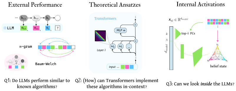
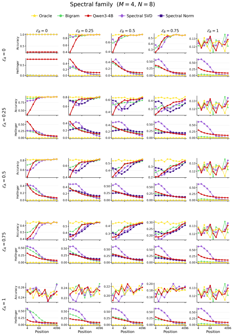
Summary. The paper proposes a three-stage approach to identify the algorithm implemented by pretrained LLMs when predicting next observations from HMM sequences. Stage 1 benchmarks 12 LLMs against classical and learning-based HMM predictors across 75 configurations and finds that no single baseline matches LLM behavior everywhere, narrowing the candidate space to Linear n-gram, Non-linear n-gram, and Spectral classes. Stage 2 gives theoretical Transformer constructions for all three classes, unified through a nonlinear-feature representation, and reports that a small Transformer trained on a single HMM converges to a finite-window linear n-gram predictor. Stage 3 introduces the Principal Activations Probe (PAP), a PCA+ridge probing method with causal activation patching, and applies it to Qwen3-1.7B. The paper concludes that pre-trained LLMs do not implement statistically optimal iterative inference, but instead use finite-window, gradient-descent-like Soft n-gram approximations, and that PAP causal interventions establish this. The manuscript is extensive and contains a large amount of empirical and theoretical material, but the central conclusion depends on claims about the Soft n-gram representation that are not fully supported by the evidence presented.
Significance. If the central claim were fully supported, the paper would be a significant step toward mechanistic identification of in-context learning algorithms in LLMs, offering a template (behavioral comparison + theoretical constructions + probing + causal intervention) that could transfer to other algorithmic families. The paper has genuine strengths: a broad and systematic empirical comparison; explicit Transformer constructions for several algorithmic classes; a carefully validated small-Transformer experiment; and a probing method with null tests, multiple patch types, and cross-model-size checks. These components are valuable and likely reusable. However, the headline conclusion about finite-window Soft n-gram inference in pre-trained LLMs is currently underdetermined by the PAP results, for the reasons detailed in the major comments. The disconnect between the strong conclusion and the fragility of the causal identification is the main gap between the paper's potential and its current form.
major comments (4)
- [§4.2 / Table 2 / App. B.3] The 'Soft n-gram belief' r_t = W_t z_t is not a finite-window quantity. Appendix B.3 states that for the Soft n-gram entry, Ridge MSE weights are used: W_t is the closed-form ridge solution fit on the full prefix o_{1:t-1}. Thus r_t depends on the entire context through W_t, and only the feature z_t is finite-window. Patching r_t^{tgt} via Eq. (4) therefore transfers full-context information from the target sequence. The observed causal efficacy is consistent with the model using long-range information encoded in W_t, and does not identify a finite-window mechanism. The Bigram control does not control for this because Bigram has no full-context adaptive operator. This directly undermines the central claim in Section 6 that LLMs use 'finite-window, gradient-descent-like' inference.
- [§3.1 / Lemma C.1] Lemma 3.1/Lemma C.1 does not support the statement that the prediction problem 'reduces to learning a linear operator.' In Eq. (11), the matrix G_{t,n} depends on t through the unobserved belief b_{t-n} and the normalizer α_{t,n}. A fixed linear matrix W such that q_{t+1} ≈ W φ_t is an approximation, not an exact reduction. Theorem 3.2 shows that a Transformer can emulate gradient descent on a fixed logistic-regression parameter, but does not show that the resulting W approximates the time-varying Bayes-optimal G_{t,n}. The manuscript should state this approximation explicitly, characterize its error, and identify regimes where it is accurate; otherwise the theoretical grounding for the 'Soft n-gram' class as a candidate algorithm is incomplete.
- [§4.1, Eq. (4)] The probe-inverse patch for Soft n-gram writes an N-dimensional next-token distribution (W_t z_t) into the residual stream, whereas the Oracle patch targets an M-dimensional hidden-state belief. Because the Soft n-gram target is, by construction, a predictor of the next token, high IIA may merely reflect that the model's output is linearly writable from the residual stream, not that the algorithm's internal state is being used. A discriminating control should patch a fixed finite-window n-gram distribution with no full-context operator, or compare IIA against the Oracle belief with matched dimensionality. Without such a control, the causal identification of Soft n-gram as the operative algorithm is fragile.
- [§6 / §3.2] The conclusion that LLMs use 'gradient-descent-like' approximations is not supported by the pretrained-LLM experiments. The PAP target for Soft n-gram uses Ridge MSE (closed-form ridge regression), not online gradient descent; the only evidence of gradient-descent-like behavior comes from the small-Transformer experiment in Section 3.2, which trains on a single fixed HMM and does not address pre-trained models. The conclusion should distinguish between the small-Transformer finding and the pretrained-LLM finding, and either provide direct evidence for online GD in pretrained LLMs or soften the claim.
minor comments (4)
- [Abstract / §1] The abstract says PAP 'reveals low-dimensional linear representations that causally drive model predictions'; for Soft n-gram the target r_t is N-dimensional, so 'low-dimensional' should be qualified or the PCA dimension should be made explicit.
- [§2.3] The empirical comparison reports no error bars or confidence intervals. Given the checklist claims closed-form linear regression for crucial experiments, adding error bars for the behavioral comparisons would strengthen the claims.
- [Appendix B.3] Ridge regularization λ is said to be selected on a held-out validation split, but no details are given on the sweep or the criterion. Please specify.
- [Appendix D] The Neumann-series approximation for f_bi requires conditions on the spectral radius of (I - U^T P_2,1); these conditions are not stated. Since this is part of a capability construction rather than the main empirical claim, this is a clarity issue, not a blocking one.
Circularity Check
The Soft n-gram 'belief' probed by PAP is a full-context ridge-regression fit expressed as next-token logits, so the headline 'finite-window, gradient-descent-like' conclusion is partly forced by construction.
specific steps
-
fitted input called prediction
[Appendix B.3 (Ridge MSE) + Section 4.2, Table 2 (Soft n-gram belief definition)]
"Ridge MSE. At each evaluation position, we solve the closed-form ridge regression ... and predict qt+1 = Ŵtψ(n)t ... For the Soft n-gram entry of Table 2 (Section 4), we use Ridge MSE weights at position t: the operator representation is Wt and the belief representation is Wtψ(n)t."
The probed 'algorithmic belief' r_t = W_t z_t is the output of a regressor fit on the entire prefix o_{1:t} via closed-form ridge regression, so it is a full-context fitted next-token predictor, not a finite-window internal state. The causal test then patches this already output-space, N-dimensional logit vector through probe-inverse Eq. (4) and scores agreement with the 'expected next-token distribution under r_t^tgt' — i.e., against the very distribution the ridge fit was optimized to produce. High IIA is therefore expected whenever the LLM's output is linearly writable from the residual stream and near the Bayes-optimal predictor that the ridge fit also approximates; it does not establish that the model computes Soft n-gram, and it cannot support the finite-window part of the conclusion
-
self definitional
[Section 4.2 (Soft n-gram definition) vs. Section 6 (central conclusion)]
"For Soft n-gram, the belief is the predicted logit Wtzt, where zt ∈ {ψ(n)t , ϕ(n)t } is the finite-window feature from Lemma 3.1 and Wt ∈ R^{N×dim(zt)} is the in-context learned weight... The central conclusion is that LLMs ... appear to learn finite-window, gradient-descent-like approximations well-described by Soft n-gram statistics."
The paper attaches the label 'finite-window' to the whole belief W_t z_t based solely on the feature z_t, while W_t is refit from the full observation prefix; the probed object therefore encodes long-range context. The headline 'finite-window' conclusion is obtained by definitionally assigning the finite-window property to the feature and ignoring the full-context weight. Moreover, even the theoretical n-gram map in Lemma 3.1 / Appendix C.1 has G_{t,n} depending on the long-history belief b_{t-n}, so the finite-window characterization is built into the naming of the representation rather than derived from it.
full rationale
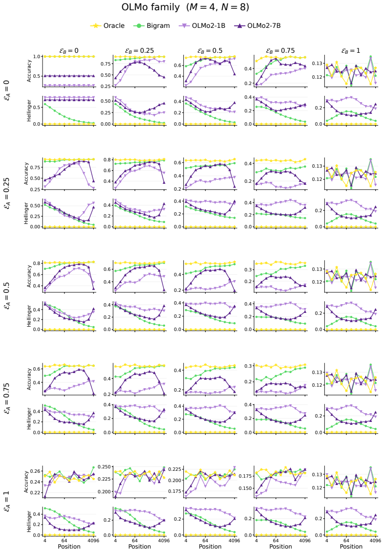
The paper contains substantial non-circular content: the empirical benchmark against HMM baselines, the Transformer implementation constructions (Lemmas 3.1, C.1–C.6 and Theorem 3.2), and the small trained Transformer analysis are self-contained. The PAP method itself is standard probing plus activation patching, and the Oracle-belief results, including the OLMo contrast, are independent evidence. However, the central mechanistic claim for pre-trained LLMs — that they use finite-window, gradient-descent-like Soft n-gram inference — rests on a target representation that is partly circular. The Soft n-gram belief is defined as W_t z_t with W_t obtained by ridge regression over the whole prefix, so it is not a finite-window quantity; calling it finite-window is a definitional labeling decision. Furthermore, since the target is already an N-dimensional next-token logit vector, the probe-inverse patch that writes r_t^{tgt} and evaluates against p_{t+1}^{tgt} under r_t^{tgt} is closer to writing output logits than to intervening on an M-dimensional hidden belief, making the resulting causal effectiveness expected by construction whenever the model's output is linearly writable. The Bigram control does not repair this asymmetry, because Bigram is behaviorally far from the model in the belief-dominated regime while the ridge-refit Soft n-gram is, by construction, fit to predict next tokens from the full context. The self-citation [10] for 'LLMs converge to Bayes-optimal predictor' is not flagged as load-bearing because this paper re-derives the convergence empirically in its own experiments. Overall, partial circularity in the key causal identification warrants a score of 6 rather than a higher score, because the theoretical and small-Transformer contributions stand independently.
Axiom & Free-Parameter Ledger
free parameters (3)
- PCA rank k for PAP probes =
k=8 for main causal results; swept k ∈ {4,8,16,32,64,128,2048}
- n-gram window n for Soft n-gram =
n=4 in main probing; n=6 in small-Transformer analysis
- Ridge regularization λ =
Not reported; selected on a held-out validation split per position
axioms (4)
- domain assumption HMM stationarity, Markov property, output independence, ergodicity, and real positive transition eigenvalues
- ad hoc to paper G_{t,n} in Lemma 3.1 is learnable as a single linear operator from observation prefixes
- standard math Transformer constructions may use idealized hard attention and universal approximation of smooth maps
- domain assumption The three surviving algorithm classes (Linear n-gram, Non-linear n-gram, Spectral) are exhaustive for LLM behavior
invented entities (1)
-
Soft n-gram belief/operator representation (W_t z_t, W_t)
independent evidence
read the original abstract
Large language models (LLMs) display a striking ability to predict next observations from Hidden Markov Models (HMMs) via in-context learning (ICL), but the algorithm underlying this capability remains undetermined: prior work has proposed several candidates without consensus, and none has been grounded in the model's internal activations. We close this gap with a three-stage pipeline. First, we empirically compare LLM behavior against a suite of candidate algorithms and narrow the space to three classes -- though no single class explains LLM behavior across all HMM settings and sequence lengths. Second, we derive theoretical connections between the three classes and show how each can be implemented in-context by a Transformer, validating the construction in a small trained Transformer. Third, returning to pre-trained LLMs, we introduce the Principal Activations Probe (PAP), a layer-wise probing and intervention method that isolates algorithmic signals in model activations. PAP reveals low-dimensional linear representations that causally drive model predictions and track empirical ICL performance. PAP further reveals how these representations shift with properties of the underlying HMM regime; distinct computational stages are localized to different layers. Together, our results connect the in-context behavior of pre-trained LLMs to the underlying internal mechanisms and advance our understanding of how LLMs perform ICL on HMMs.
Figures









Reference graph
Works this paper leans on
-
[1]
Fine-grained analysis of sentence embeddings using auxiliary prediction tasks
Yossi Adi, Einat Kermany, Yonatan Belinkov, Ofer Lavi, and Yoav Goldberg. Fine-grained analysis of sentence embeddings using auxiliary prediction tasks. InInternational Conference on Learning Representations, 2017. URLhttps://openreview.net/forum?id=BJh6Ztuxl
2017
-
[2]
Transformers as implicit state estimators: In-context learning in dynamical systems.Transactions on Machine Learning Research, 2026
Usman Akram and Haris Vikalo. Transformers as implicit state estimators: In-context learning in dynamical systems.Transactions on Machine Learning Research, 2026. ISSN 2835-8856. URLhttps://openreview.net/forum?id=hIMK5MvGkP
2026
-
[3]
What learning algorithm is in-context learning? investigations with linear models
Ekin Akyürek, Dale Schuurmans, Jacob Andreas, Tengyu Ma, and Denny Zhou. What learning algorithm is in-context learning? investigations with linear models. InThe Eleventh Inter- national Conference on Learning Representations, 2023. URL https://openreview.net/ forum?id=0g0X4H8yN4I
2023
-
[4]
Understanding intermediate layers using linear classifier probes, 2017
Guillaume Alain and Yoshua Bengio. Understanding intermediate layers using linear classifier probes, 2017. URLhttps://openreview.net/forum?id=ryF7rTqgl
2017
-
[5]
Transformers as statisticians: Provable in-context learning with in-context algorithm selection
Yu Bai, Fan Chen, Huan Wang, Caiming Xiong, and Song Mei. Transformers as statisticians: Provable in-context learning with in-context algorithm selection. InThirty-seventh Conference on Neural Information Processing Systems, 2023. URL https://openreview.net/forum? id=liMSqUuVg9
2023
-
[6]
A maximization technique occurring in the statistical analysis of probabilistic functions of markov chains.The annals of mathematical statistics, 41(1):164–171, 1970
Leonard E Baum, Ted Petrie, George Soules, and Norman Weiss. A maximization technique occurring in the statistical analysis of probabilistic functions of markov chains.The annals of mathematical statistics, 41(1):164–171, 1970
1970
-
[7]
Probing classifiers: Promises, shortcomings, and advances.Computational Linguistics, 48(1):207–219, 2022
Yonatan Belinkov. Probing classifiers: Promises, shortcomings, and advances.Computational Linguistics, 48(1):207–219, 2022
2022
-
[8]
What you can cram into a single $&!#* vector: Probing sentence embeddings for linguistic properties
Alexis Conneau, German Kruszewski, Guillaume Lample, Loïc Barrault, and Marco Baroni. What you can cram into a single $&!#* vector: Probing sentence embeddings for linguistic properties. In Iryna Gurevych and Yusuke Miyao, editors,Proceedings of the 56th Annual Meeting of the Association for Computational Linguistics (Volume 1: Long Papers), pages 2126–21...
-
[9]
Cover and Joy A
Thomas M. Cover and Joy A. Thomas.Elements of Information Theory (Wiley Series in Telecom- munications and Signal Processing). Wiley-Interscience, USA, 2006. ISBN 0471241954
2006
-
[10]
Yijia Dai, Zhaolin Gao, Yahya Sattar, Sarah Dean, and Jennifer J. Sun. Pre-trained large language models learn to predict hidden markov models in-context. InThe Thirty-ninth Annual Conference on Neural Information Processing Systems, 2026. URL https://openreview. net/forum?id=btBqWTbf6q
2026
-
[11]
Transformers learn latent mixture models in-context via mirror descent
Francesco D’Angelo and Nicolas Flammarion. Transformers learn latent mixture models in-context via mirror descent. InThe Fourteenth International Conference on Learning Repre- sentations, 2026. URLhttps://openreview.net/forum?id=SHidElLSVt
2026
-
[12]
Edelman, eran malach, and Surbhi Goel
Ezra Edelman, Nikolaos Tsilivis, Benjamin L. Edelman, eran malach, and Surbhi Goel. The evolution of statistical induction heads: In-context learning markov chains. InThe Thirty- eighth Annual Conference on Neural Information Processing Systems, 2024. URL https: //openreview.net/forum?id=qaRT6QTIqJ
2024
-
[13]
Chanakya Ekbote, Marco Bondaschi, Nived Rajaraman, Jason D Lee, Michael Gastpar, Ashok Vardhan Makkuva, and Paul Pu Liang. What one cannot, two can: Two-layer trans- formers provably represent induction heads on any-order markov chains.arXiv preprint arXiv:2508.07208, 2025
arXiv 2025
-
[14]
A mathematical framework for transformer circuits.Transformer Circuits Thread,
Nelson Elhage, Neel Nanda, Catherine Olsson, Tom Henighan, Nicholas Joseph, Ben Mann, Amanda Askell, Yuntao Bai, Anna Chen, Tom Conerly, Nova DasSarma, Dawn Drain, Deep Ganguli, Zac Hatfield-Dodds, Danny Hernandez, Andy Jones, Jackson Kernion, Liane Lovitt, Kamal Ndousse, Dario Amodei, Tom Brown, Jack Clark, Jared Kaplan, Sam McCandlish, and Chris Olah. A...
-
[15]
Y . Ephraim and N. Merhav. Hidden markov processes.IEEE Transactions on Information Theory, 48(6):1518–1569, 2002. doi: 10.1109/TIT.2002.1003838
Pith/arXiv arXiv 2002
-
[16]
What can transformers learn in-context? a case study of simple function classes
Shivam Garg, Dimitris Tsipras, Percy Liang, and Gregory Valiant. What can transformers learn in-context? a case study of simple function classes. In Alice H. Oh, Alekh Agarwal, Danielle Belgrave, and Kyunghyun Cho, editors,Advances in Neural Information Processing Systems,
-
[17]
Causal abstractions of neural networks
Atticus Geiger, Hanson Lu, Thomas F Icard, and Christopher Potts. Causal abstractions of neural networks. In A. Beygelzimer, Y . Dauphin, P. Liang, and J. Wortman Vaughan, editors, Advances in Neural Information Processing Systems, 2021. URL https://openreview.net/ forum?id=RmuXDtjDhG
2021
-
[18]
Finding alignments between interpretable causal variables and distributed neural representations
Atticus Geiger, Zhengxuan Wu, Christopher Potts, Thomas Icard, and Noah Goodman. Finding alignments between interpretable causal variables and distributed neural representations. In Francesco Locatello and Vanessa Didelez, editors,Proceedings of the Third Conference on Causal Learning and Reasoning, volume 236 ofProceedings of Machine Learning Research, p...
2024
-
[19]
Hidden markov models: Pitfalls and opportunities in ecology.Methods in Ecology and Evolution, 14(1):43–56, 2023
Richard Glennie, Timo Adam, Vianey Leos-Barajas, Théo Michelot, Theoni Photopoulou, and Brett T McClintock. Hidden markov models: Pitfalls and opportunities in ecology.Methods in Ecology and Evolution, 14(1):43–56, 2023
2023
-
[20]
Yifan Hao, Chenlu Ye, Chi Han, and Tong Zhang. Transformers as multi-task learners: Decou- pling features in hidden markov models.arXiv preprint arXiv:2506.01919, 2025
Pith/arXiv arXiv 2025
-
[21]
A spectral algorithm for learning hidden markov models.Journal of Computer and System Sciences, 78(5):1460–1480, 2012
Daniel Hsu, Sham M Kakade, and Tong Zhang. A spectral algorithm for learning hidden markov models.Journal of Computer and System Sciences, 78(5):1460–1480, 2012
2012
-
[22]
On limitation of transformer for learning hmms.arXiv preprint arXiv:2406.04089, 2024
Jiachen Hu, Qinghua Liu, and Chi Jin. On limitation of transformer for learning hmms.arXiv preprint arXiv:2406.04089, 2024
Pith/arXiv arXiv 2024
-
[23]
Visualisation and ’diagnostic classifiers’ reveal how recurrent and recursive neural networks process hierarchical structure (extended abstract)
Dieuwke Hupkes and Willem Zuidema. Visualisation and ’diagnostic classifiers’ reveal how recurrent and recursive neural networks process hierarchical structure (extended abstract). InPro- ceedings of the Twenty-Seventh International Joint Conference on Artificial Intelligence, IJCAI- 18, pages 5617–5621. International Joint Conferences on Artificial Intel...
-
[24]
On the origins of linear representations in large language models
Yibo Jiang, Goutham Rajendran, Pradeep Kumar Ravikumar, Bryon Aragam, and Victor Veitch. On the origins of linear representations in large language models. InForty-first International Conference on Machine Learning, 2024. URL https://openreview.net/ forum?id=otuTw4Mghk
2024
-
[25]
Emergent world models and latent variable estimation in chess-playing lan- guage models
Adam Karvonen. Emergent world models and latent variable estimation in chess-playing lan- guage models. InFirst Conference on Language Modeling, 2024. URL https://openreview. net/forum?id=PPTrmvEnpW
2024
-
[26]
Li, Zifan Carl Guo, and Jacob Andreas
Belinda Z. Li, Zifan Carl Guo, and Jacob Andreas. (how) do language models track state? InForty-second International Conference on Machine Learning, 2025. URL https://openreview.net/forum?id=8SXosAVIFH
2025
-
[27]
Emergent world representations: Exploring a sequence model trained on a synthetic task
Kenneth Li, Aspen K Hopkins, David Bau, Fernanda Viégas, Hanspeter Pfister, and Martin Wattenberg. Emergent world representations: Exploring a sequence model trained on a synthetic task. InThe Eleventh International Conference on Learning Representations, 2023. URL https://openreview.net/forum?id=DeG07_TcZvT
2023
-
[28]
From kepler to newton: Inductive biases guide learned world models in transformers, 2026
Ziming Liu, Sophia Sanborn, Surya Ganguli, and Andreas Tolias. From kepler to newton: Inductive biases guide learned world models in transformers, 2026. URL https://arxiv. org/abs/2602.06923
arXiv 2026
-
[29]
Xiaoyuan Ma and Jordan Rodu. Bridging the usability gap: Theoretical and methodological advances for spectral learning of hidden markov models.arXiv preprint arXiv:2302.07437, 2023. 13
Pith/arXiv arXiv 2023
-
[30]
Attention with markov: A curious case of single-layer transformers
Ashok Vardhan Makkuva, Marco Bondaschi, Adway Girish, Alliot Nagle, Martin Jaggi, Hyeji Kim, and Michael Gastpar. Attention with markov: A curious case of single-layer transformers. InThe Thirteenth International Conference on Learning Representations, 2025. URL https: //openreview.net/forum?id=SqZ0KY4qBD
2025
-
[31]
Uncovering ecological state dynamics with hidden markov models.Ecology letters, 23(12):1878–1903, 2020
Brett T McClintock, Roland Langrock, Olivier Gimenez, Emmanuelle Cam, David L Borchers, Richard Glennie, and Toby A Patterson. Uncovering ecological state dynamics with hidden markov models.Ecology letters, 23(12):1878–1903, 2020
1903
-
[32]
Progress mea- sures for grokking via mechanistic interpretability
Neel Nanda, Lawrence Chan, Tom Lieberum, Jess Smith, and Jacob Steinhardt. Progress mea- sures for grokking via mechanistic interpretability. InThe Eleventh International Conference on Learning Representations, 2023. URL https://openreview.net/forum?id=9XFSbDPmdW
2023
-
[33]
Emergent linear representations in world models of self-supervised sequence models
Neel Nanda, Andrew Lee, and Martin Wattenberg. Emergent linear representations in world models of self-supervised sequence models. In Yonatan Belinkov, Sophie Hao, Jaap Jumelet, Na- joung Kim, Arya McCarthy, and Hosein Mohebbi, editors,Proceedings of the 6th BlackboxNLP Workshop: Analyzing and Interpreting Neural Networks for NLP, pages 16–30, Singapore, ...
-
[34]
Riechers, Daniel Filan, and Adam Shai
Mateusz Piotrowski, Paul M. Riechers, Daniel Filan, and Adam Shai. Constrained belief updates explain geometric structures in transformer representations. InForty-second Interna- tional Conference on Machine Learning, 2025. URL https://openreview.net/forum? id=f6Hl60FBFU
2025
-
[35]
Transformers on markov data: Constant depth suffices
Nived Rajaraman, Marco Bondaschi, Ashok Vardhan Makkuva, Kannan Ramchandran, and Michael Gastpar. Transformers on markov data: Constant depth suffices. InICML 2024 Workshop on Mechanistic Interpretability, 2024. URL https://openreview.net/forum? id=jnCM5EHd2H
2024
-
[36]
Yahya Sattar, Yassir Jedra, Maryam Fazel, and Sarah Dean. Finite sample identification of partially observed bilinear dynamical systems.arXiv preprint arXiv:2501.07652, 2025
arXiv 2025
-
[37]
URLhttps://aclanthology.org/2023.blackboxnlp-1.2/
2023
-
[38]
Chang, Ashesh Rambachan, and Sendhil Mullainathan
Keyon Vafa, Peter G. Chang, Ashesh Rambachan, and Sendhil Mullainathan. What has a foundation model found? inductive bias reveals world models. InForty-second Interna- tional Conference on Machine Learning, 2025. URL https://openreview.net/forum? id=i9npQatSev
2025
-
[39]
Aditya Varre, Gizem Yüce, and Nicolas Flammarion. Learning in-context n-grams with transformers: Sub-n-grams are near-stationary points.arXiv preprint arXiv:2508.12837, 2025
Pith/arXiv arXiv 2025
-
[40]
Itay Yona, Ilia Shumailov, Jamie Hayes, Federico Barbero, and Yossi Gandelsman. Interpreting the repeated token phenomenon in large language models.arXiv preprint arXiv:2503.08908, 2025
Pith/arXiv arXiv 2025
-
[41]
Riechers, Lucas Teixeira, Alexander Gietelink Oldenziel, and Sarah Marzen
Adam Shai, Paul M. Riechers, Lucas Teixeira, Alexander Gietelink Oldenziel, and Sarah Marzen. Transformers represent belief state geometry in their residual stream. InThe Thirty- eighth Annual Conference on Neural Information Processing Systems, 2024. URL https: //openreview.net/forum?id=YIB7REL8UC
2024
-
[42]
A hidden markov model for space-time precipitation.Water Resources Research, 27(8):1917–1923, 1991
Walter Zucchini and Peter Guttorp. A hidden markov model for space-time precipitation.Water Resources Research, 27(8):1917–1923, 1991. 14 Appendices Table of Contents • Appendix A: Additional HMM Background • Appendix B: Benchmark Algorithmic Details • Appendix C:n-gram Prediction Constructions • Appendix E: Details of the Small Trained Transformer • Appe...
1917
-
[45]
Fred Zhang and Neel Nanda. Towards best practices of activation patching in language models: Metrics and methods.arXiv preprint arXiv:2309.16042, 2023
Pith/arXiv arXiv 2023
-
[47]
Initialize eb1 =f uni(o1:t)
-
[48]
, t−1: • Set eb′ k =f tri(o1:t, ebk, ok)
Fork= 1, . . . , t−1: • Set eb′ k =f tri(o1:t, ebk, ok). • Set ebk+1 =f bi(o1:t, eb′ k). After this loop, ebt is the updated belief after processingo 1, . . . , ot−1
-
[49]
• Setc o =f bi(o1:t, ebo t+1)
For eacho∈ O: • Set ebo t+1 =f tri(o1:t, ebt, o). • Setc o =f bi(o1:t, ebo t+1)
-
[50]
Normalize overo∈ O
Output for symbol o: eb⊤ ∞co, where eb∞ = (P ⊤ 2,1U) +P1 is the fixed terminal vector from the observable representation defined above. Normalize overo∈ O. We now argue that each primitive and their composition can be approximated by a Transformer. 24 Approximating funi.Since P1 =E[u t] and U is a fixed matrix (estimated once from the prefix via SVD of bP...
2048
-
[51]
We need at least (32, 128), and increasing beyond (64,256) does not lead to better performance
and (16, 64), we can see underfitting based on training and validation loss. We need at least (32, 128), and increasing beyond (64,256) does not lead to better performance. 26 0 500 1000 1500 Step 2.1 2.2 2.3 2.4Training Loss Training Loss 0 500 1000 1500 Step 2.1 2.2 2.3 2.4Validation Loss Validation Loss 2 4 8 16326412825651210242048 Location 0.275 0.30...
2049
-
[53]
Guidelines: • The answer [N/A] means that the paper does not involve crowdsourcing nor research with human subjects
Institutional review board (IRB) approvals or equivalent for research with human subjects Question: Does the paper describe potential risks incurred by study participants, whether such risks were disclosed to the subjects, and whether Institutional Review Board (IRB) approvals (or an equivalent approval/review based on the requirements of your country or ...
-
[2018]
URL https://doi.org/10.24963/ijcai.2018/796
doi: 10.24963/ijcai.2018/796. URL https://doi.org/10.24963/ijcai.2018/796
-
[2021]
https://transformer-circuits.pub/2021/framework/index.html. 12
2021
-
[2022]
URLhttps://openreview.net/forum?id=flNZJ2eOet
-
[4096]
AAAA
The OLMo family (OLMo2-1B, OLMo2-7B) performs the worst overall: it degrades markedly at longer context lengths (T∈ {1024,2048,4096}), exhibiting a pronounced U-shaped trend, and underperforms other families when either transition or emission entropies is high. 31 Qwen family (M = 4, N = 2) Oracle Bigram Qwen2.5-1.5B Qwen3-0.6B Qwen3-1.7B Qwen3-4B Qwen3-8...
2048
discussion (0)
Sign in with ORCID, Apple, or X to comment. Anyone can read and Pith papers without signing in.