REVIEW 3 major objections 4 minor 25 references
Force Geometry and Irreversibility in Nonequilibrium Overdamped Dynamics
T0 review · 3 major / 4 minor · reviewed 2026-08-02 · deepseek-v4-flash
Pith's one-line read For overdamped systems, entropy production is determined by the relative orientation of driving and entropic forces, vanishing only at exact anti-alignment; a new correlation coefficient provides a geometric lower bound and a thermodynamic
desk verdict Correct harmonic-trap geometry, but the general stall condition and the RBC membrane mapping are overclaims. read the letter →
The pith
A machine-rendered reading of the paper's core claim, the machinery that carries it, and where it could break.
The reading
What carries the argument
The central object is the decomposition of the net thermodynamic force into external and entropic parts, F_net = F_ext + F_info, with F_ext = -∇U and F_info = -k_B T ∇ ln ρ. Through the identity Ṡ_i = (D/k_B T²)⟨F_net²⟩, the entropy production rate splits into force variances plus a cross-term, which is normalized into the force-correlation coefficient r(t) = ⟨F_ext F_info⟩/√(⟨F_ext²⟩⟨F_info²⟩). This coefficient turns the quadratic form into a geometric statement about orientation. The moving harmonic trap supplies the solvable case where both forces are linear but centered at different points; the resulting r = -σ/√(σ² + Δ²) maps directly to control charts, and the bound saturation at r =
What would settle it
In a single trapped bead dragged at constant velocity, measure entropy production (e.g., via heat dissipation or a variance sum rule) together with σ and Δ across a range of stiffnesses and velocities. The theory predicts the exact collapse Ṡ k_B T²/D = k²(σ²+Δ²) + (k_B T)²/σ² − 2k k_B T, with r = −σ/√(σ²+Δ²). A systematic deviation from this surface, or a measured entropy production below the geometric bound, would falsify the central claim.
Extended reading notes
Core claim
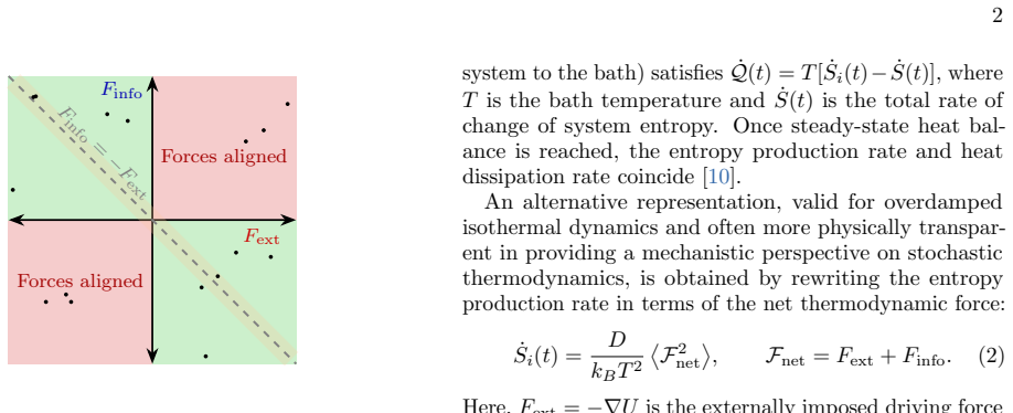
Entropy production in overdamped dynamics is not fixed by force magnitudes alone; it depends on the alignment between the driving force F_ext and the entropic force F_info = -k_B T ∇ ln ρ. From the identity Ṡ_i = (D/k_B T²)⟨(F_ext + F_info)²⟩, a correlation coefficient r(t) quantifies the cross-term and sets how much dissipation arises for given force scales. Perfect pointwise anti-alignment makes entropy production vanish; global anti-alignment (r = -1) is a thermodynamic stall where mean transport stops but entropy production stays finite. The bound Ṡ_i ≥ (D/k_B T²)(√⟨F_ext²⟩ - √⟨F_info²⟩)² is saturated at stall. For a harmonic trap, r = -σ/√(σ² + Δ²), so the ratio |Δ|/σ governs dissipat
Load-bearing premise
The paper assumes that each membrane patch behaves as a single overdamped harmonic oscillator with well-defined stiffness, friction, and temperature, so that measured variance and lag determine r; that mapping is asserted without evidence.
Editorial extensions
If this is right
- In overdamped harmonic traps, entropy production is fixed by the ratio |Δ|/σ of lag to fluctuations, so two easily measured quantities determine dissipation.
- Thermodynamic stall is distinct from reversibility: at r = -1 transport vanishes but entropy production can remain finite, so a zero-current measurement does not imply equilibrium.
- Protocols can reduce dissipation at fixed transport by tuning stiffness and velocity to improve anti-alignment; constant-alignment contours obey k ∝ v².
- For sinusoidal driving, time-averaged force correlation and injected power both depend on Q sin²φ, so constant-cost contours coincide with constant-alignment contours.
- The framework explains why high-fluctuation regions can be low-dissipation: they may operate near perfect anti-alignment, buffering energetic cost.
Reading between the lines
- If the harmonic-trap mapping holds, the same variance–lag construction could serve as a non-invasive probe of local force organization in any driven soft-matter system, using only position time series to estimate r and the distance to stall.
- The control-chart reasoning suggests a biological design principle: cells may suppress metabolic dissipation by orchestrating internal forces to nearly cancel external loads while preserving activity, exactly the regime hinted at by membrane experiments.
- The underdamped extension implies a possible 'coasting' regime where positional anti-alignment coexists with directed transport; testing this in micro-mechanical oscillators would directly probe whether inertia decouples force geometry from transport.
- A sharper stall diagnostic could be built by measuring the variance of the net force, since the paper's equations give Ṡ_i ∝ Var(F_net) when r = -1; verifying this would isolate the stall regime in experiments.
Signed reviews
Editorial analysis
A structured set of objections, weighed in public.
Referee Report
Summary. The paper proposes a force-geometric decomposition of entropy production in overdamped Langevin dynamics. It defines a force–correlation coefficient r(t) between the external driving force and the information-theoretic (entropic) force, derives an instantaneous lower bound on the entropy production rate, and claims that r = −1 defines a thermodynamic stall condition with vanishing mean transport but finite entropy production. Exact results for moving harmonic traps under constant drag and sinusoidal driving are used to construct 'geometric control charts', and the framework is applied as a structural explanation of the fluctuation–dissipation anticorrelation observed in red-blood-cell membrane experiments.
Significance. The exact harmonic-trap calculations (Eqs. (8)–(9), (10)–(12), SM III–V) are internally correct, self-contained, and involve no fitted parameters; the Cauchy–Schwarz lower bound in Eq. (5) is a genuine mathematical identity. These are useful benchmark results. However, the central conceptual claims—that r = −1 defines thermodynamic stall and that the control charts quantify thermodynamic cost—are not supported by those calculations, and the experimental application rests on an unvalidated model assumption. As written, the advertised 'force geometry as an organizing principle' is not established at the level claimed.
major comments (3)
- [Force Geometry and Entropy Production, Eq. (4)] The definition of r in Eq. (4) is an uncentered product-moment. Equality r = −1 means F_info = a F_ext with a < 0 (Cauchy–Schwarz equality), not that ⟨F_net⟩ = 0. For any a < 0, a ≠ −1, the configuration F_info = a F_ext gives r = −1 but ⟨F_net⟩ = (1+a)⟨F_ext⟩, generally nonzero, and Eq. (2) gives Ṡ_i > 0. Such a state is realizable in overdamped dynamics (e.g. ρ ∝ exp(aU/k_BT) on a bounded domain). Hence the sentence after Eq. (4) and the stall row of Fig. 2 are false in general. In the exact harmonic-trap model, Eq. (9) yields r = −1 only at Δ = 0, i.e. equilibrium with Ṡ_i = 0, so the advertised 'stall with Ṡ_i > 0' is not exhibited by the paper's own example.
- [Geometric organization and experimental operating regimes, Eq. (10), Fig. 5] For constant-velocity dragging, the steady-state entropy production rate is Ṡ_i = γv²/T, independent of k: from Eq. (8), ⟨F_net²⟩ = γ²v², and Ṡ_i = D⟨F_net²⟩/(k_BT²). Thus at fixed transport speed v, varying k changes r_ss but does not change dissipation. The sentence 'Operating points with r_ss closer to −1 correspond to ... reduced dissipation at fixed transport speed' is therefore incorrect; only the lower bound Eq. (5) decreases, and it is not tight for r_ss > −1. Consequently, Fig. 5's claim that families of protocols with identical power input have 'distinct thermodynamic costs' is misleading: in steady state the thermodynamic cost is P/T = γv²/T.
- [Experimental connection and geometric explanation, Fig. 5, SM VI] The mapping of each red-blood-cell membrane patch to an overdamped harmonic trap is asserted, not derived. The lag Δ and the effective stiffness/friction are not independently measured in Ref. [2]; the passive flicker data do not establish linear, Markovian, isothermal, single-temperature patch dynamics. Moreover, the rescaling to the reference friction γ0 = 0.01 pN·s/µm shifts r from −0.91 (using γ_exp = 0.025 pN·s/µm) to −0.96 (SM VI), a change that is material to the 'strong anti-alignment' interpretation. If the harmonic-trap analogy fails, the claimed geometric explanation of the fluctuation–dissipation anticorrelation and the control-chart placement do not follow.
minor comments (4)
- [Force Geometry and Entropy Production, Eq. (4)] If the quantity is meant to be a Pearson correlation coefficient, it should be defined with centered random variables. The uncentered version is not invariant to adding constants to the forces, and this nonstandard choice is directly connected to Major Comment 1.
- [References, Ref. [12]] The central derivation in SM I cites Ref. [12] as 'in preparation'. The derivation is short and is already sketched; it should either be completed in the paper or the reference should be replaced by a published source.
- [Fig. 5 caption and SM VI] The yellow star in Fig. 5 corresponds to r ≈ −0.96 after rescaling to γ0 = 0.01 pN·s/µm, while the directly measured parameters give r ≈ −0.91. The main text should state this distinction at the point of the claim, rather than only in the SM.
- [Sinusoidal driving, Eq. (11)] The complete elliptic integral K is written with a negative parameter. To avoid ambiguities between the K(m) and K(k) conventions, the convention should be specified in the text or in a footnote.
Circularity Check
No significant circularity: the central entropy-production identity and geometric bound are derived from the Fokker–Planck equation and Cauchy–Schwarz, and the experimental applications are illustrative mappings rather than fitted predictions.
full rationale
The derivation chain is self-contained. Eq. (2) is obtained in SM I by direct manipulation of the overdamped Fokker–Planck equation, so the in-preparation self-citation [12] is redundant and not load-bearing. Equations (3)–(5) are an algebraic expansion and a Cauchy–Schwarz inequality, with saturation at perfect anti-alignment following from the equality condition rather than being assumed. The harmonic-trap results (Eqs. (6)–(11); SM III–V) are solved exactly from the Ornstein–Uhlenbeck process, and the correlation coefficient r = −σ/√(Δ²+σ²) follows from Gaussian moments. The RBC operating point is mapped from reported experimental parameters (k, v, γ, T) with the rescaling disclosed; r_ss ≈ −0.91 (SM Fig. 1) and −0.96 after rescaling are calculations, not fits that determine the model constants. The only caveats—the harmonic-trap mapping of membrane patches and the in-preparation reference—are correctness/verification concerns, not circularity: no prediction in the paper reduces by construction to a fitted parameter or to an assumed version of the target result.
Assumptions & free parameters
free parameters (1)
- Reference friction coefficient γ0 =
0.01 pN·s/µm
assumptions (5)
- standard math Seifert's definition of entropy production rate from stochastic thermodynamics (including the identification of Ṡ_i = Ṡ - Ṡ_e) is the correct measure of irreversibility.
- domain assumption Overdamped Langevin dynamics with additive Gaussian white noise and the corresponding Fokker-Planck equation describe the systems of interest (optical traps, membrane patches).
- standard math For harmonic traps, a Gaussian initial distribution remains Gaussian, so the probability density is fully characterized by mean μ(t) and variance σ²(t).
- domain assumption The entropy production rate can be decomposed into an external force and an information force F_info = -k_B T ∇ ln ρ; the latter is treated as a genuine force in the geometric picture.
- standard math For sinusoidal driving, the system reaches a periodic steady state with time-independent variance σ² = k_B T/k.
Cite this review
Pith. "Pith review of Force Geometry and Irreversibility in Nonequilibrium Overdamped Dynamics." pith.science (2026). https://pith.science/paper/M5WPDSE2
@misc{pith2026260329416,
  author       = {Pith},
  title        = {Pith review of: Force Geometry and Irreversibility in Nonequilibrium Overdamped Dynamics},
  year         = {2026},
  howpublished = {\url{https://pith.science/paper/M5WPDSE2}},
  note         = {Machine review of arXiv:2603.29416}
}
read the original abstract
Recent experiments have revealed heterogeneous dissipation in optically trapped systems, often anticorrelated with local positional fluctuations, exposing a structural gap in the scalar stochastic thermodynamic description. While the scalar framework successfully quantifies dissipation through currents and entropy production rates, it does not reveal the underlying vectorial force geometry that shapes spatial dissipation patterns. Here, we bridge this gap by identifying force geometry as an organizing principle for nonequilibrium thermodynamics, introducing force alignment as a geometric determinant of irreversibility. We show that entropy production depends not only on force magnitudes but also on the relative orientation between deterministic driving forces and entropic gradients, vanishing only under exact anti-alignment with matched magnitudes. We formalize this geometric alignment through a time-dependent force-correlation coefficient, quantifying the relative orientation between the forces. This yields an instantaneous geometric lower bound on entropy production that remains valid even when force magnitudes are matched. For overdamped dynamics, perfect anti-alignment defines a thermodynamic stall where net transport vanishes and the lower bound on entropy production is saturated. This force-level perspective provides a structural explanation for the experimentally observed fluctuation-dissipation anticorrelation and nonuniform dissipation. We construct geometric control charts for both constant dragging and sinusoidal driving protocols, explicitly locating experimental operating points within this force-space representation. Together, these results position force geometry as a unifying structural perspective on irreversibility, spanning active biological systems, microrheology, and naturally extending to underdamped dynamics.
Figures


Figures from the paper (3 more)


Reference graph
Works this paper leans on
-
[2]
Di Terlizzi, M
I. Di Terlizzi, M. Gironella, D. Herraez-Aguilar, T. Betz, F. Monroy, M. Baiesi, and F. Ritort. Variance sum rule for entropy production.Science, 383(6686):971–976, 2024
2024
-
[1]
Sekimoto
K. Sekimoto. Langevin Equation and Thermodynamics. Prog. Theor. Phys. Suppl., 130:17–27, 1998
1998
-
[3]
Di Terlizzi
I. Di Terlizzi. Force-Free Kinetic Inference of Entropy Production.Phys. Rev. Lett., 135:237101, 2025
2025
-
[4]
A. C. Barato and U. Seifert. Thermodynamic Uncertainty Relation for Biomolecular Processes.Phys. Rev. Lett., 114:158101, 2015
2015
-
[5]
T. R. Gingrich, J. M. Horowitz, N. Perunov, and J. L. England. Dissipation Bounds All Steady-State Current Fluctuations.Phys. Rev. Lett., 116:120601, 2016
2016
-
[6]
U. Seifert. From Stochastic Thermodynamics to Thermo- dynamic Inference.Annu. Rev. Condens. Matter Phys., 10:171–192, 2019
2019
-
[7]
J. M. Horowitz and T. R. Gingrich. Thermodynamic un- certainty relations constrain non-equilibrium fluctuations. Nat. Phys., 16(1):15–20, 2020
2020
-
[8]
S. B. Nicholson, L. P. Garc ´ ıa-Pintos, A. del Campo, and J. R. Green. Time–information uncertainty relations in thermodynamics.Nat. Phys., 16:1211–1215, 2020
2020
Show all 25 references
-
[9]
Dechant and S.-i
A. Dechant and S.-i. Sasa. Improving Thermodynamic Bounds Using Correlations.Phys. Rev. X, 11:041061, 2021
2021
-
[10]
U. Seifert. Entropy Production along a Stochastic Tra- jectory and an Integral Fluctuation Theorem.Phys. Rev. Lett., 95:040602, 2005
2005
-
[11]
Springer Series in Synergetics
H Risken.The Fokker-Planck Equation: Methods of So- lution and Applications. Springer Series in Synergetics. Springer, Berlin, Heidelberg, 2 edition, 1996
1996
-
[12]
R. K. Singh, C. Nezat, G. Trahan, J. Gounsoulin, D. Silva, S. Das, and E. Aghion. Entropy production from the over- damped Fokker–Planck equation: A pedagogical deriva- tion. in preparation, 2026
2026
-
[13]
Jarzynski
C. Jarzynski. Nonequilibrium Equality for Free Energy Differences.Phys. Rev. Lett., 78:2690–2693, 1997
1997
-
[14]
U. Seifert. Stochastic thermodynamics, fluctuation theorems and molecular machines.Rep. Prog. Phys., 75:126001, 2012
2012
-
[15]
K. C. Neuman and S. M. Block. Optical trapping.Rev. Sci. Instrum., 75:2787–2809, 2004
2004
-
[16]
Kumar, V
R. Kumar, V. Vitali, T. Wiedemann, A. Quagliarini, R. Ferracci, F. Cordella, M. Ponzini, E. Zaccarelli, J. Roca- Bonet, G. Pesce, A. C. De Luca, O. M. Marag` o, and G. Volpe. Multi-frequency passive and active microrheol- ogy with optical tweezers.Sci. Rep., 11:13917, 2021
2021
-
[17]
Catal` a-Castro, S
F. Catal` a-Castro, S. Ortiz-V´ asquez, C. Mart ´ ınez- Fern´ andez, F. Pezzano, C. Garcia-Cabau, M. Fern´ andez- Campo, N. Sanfeliu-Cerd´ an, S. Jim´ enez-Delgado, X. Sal- vatella, V. Ruprecht, P.-A. Frigeri, and M. Krieg. Measur- ing age-dependent viscoelasticity of organell...
2025
-
[18]
Ito and A
S. Ito and A. Dechant. Stochastic Time Evolution, In- formation Geometry, and the Cram´ er-Rao Bound.Phys. Rev. X, 10:021056, 2020
2020
-
[19]
S. Dago, J. Pereda, N. Barros, S. Ciliberto, and L. Bel- lon. Information and Thermodynamics: Fast and Precise Approach to Landauer’s Bound in an Underdamped Mi- cromechanical Oscillator.Phys. Rev. Lett., 126:170601, 2021
2021
-
[20]
Oikawa, Y
S. Oikawa, Y. Nakayama, S. Ito, and J. Bechhoefer. Ex- perimentally achieving minimal dissipation via thermody- namically optimal transport.Nat. Commun., 16:10424, 2025
2025
-
[21]
N. G. van Kampen.Stochastic Processes in Physics and Chemistry. Elsevier, 3 edition, 2007
2007
-
[22]
Springer, 2010
Ken Sekimoto.Stochastic Energetics, volume 799 ofLec- ture Notes in Physics. Springer, 2010
2010
-
[23]
D ∂2 xρ(x, t) + D kBT ∂x U ′(x, t)ρ(x, t) # lnρ(x, t)dx − 1 T Z ∞ −∞
Richard E. Spinney and Ian J. Ford. Entropy production in full phase space for continuous stochastic dynamics. Phys. Rev. E, 85:051113, 2012. Supplemental Material: Force Geometry and Irreversibility in Nonequilibrium Dynamics Erez Aghion 1 and Swetamber Das 2 1Department of P...
2012
-
[24]
Constant input power:γ 0v2 0 =P exp,
-
[25]
Constant trap stiffness:k 0 =k exp. The rescaled velocity is therefore v0 =v exp r γexp γ0 ≈15.8µm/s.(52) This rescaling preserves the experimentally relevant en- ergy injection scale and does not alter the qualitative location of the operating point on the geometric chart. Ef...
Reviewed August 2, 2026 · model on record in the stance chip above.
Discussion (0). Continue with ORCID to comment.