Deep Learning for Dynamic Programming with Recursive Utility

Wu Guo; Xianhua Peng

REVIEW 3 major objections 4 minor 4 references

A new deep-learning method solves high-dimensional dynamic programs with recursive utility by learning the certainty equivalent itself.

Reviewed by Pith at T0; open to challenge. T0 means a machine referee read the full paper against a public rubric. the ladder, T0–T4 →

Challenge this review Re-run · record.json Download PDF Read on arXiv ↗

T0 review · grok-4.5

2026-07-11 20:25 UTC pith:MIVYPTXP

load-bearing objection Solid computational methods paper: CEL is a real design for recursive-utility DP, with strong closed-form and VFI evidence, but residual claims need a bias audit and code. the 3 major comments →

arxiv 2607.04278 v1 pith:MIVYPTXP submitted 2026-07-05 q-fin.CP cs.LGecon.EMmath.OCstat.ML

Deep Learning for Dynamic Programming with Recursive Utility

Xianhua Peng , Wu Guo This is my paper

classification q-fin.CP cs.LGecon.EMmath.OCstat.ML

keywords recursive utilitydeep learningdynamic programmingcertainty equivalentneural networksportfolio choicestrategic asset allocationEpstein–Zin preferences

verification ladder T0 review T1 audit T2 compute T3 formal T4 reserved

The pith

A machine-rendered reading of the paper's core claim, the machinery that carries it, and where it could break.

Many economic and financial decisions use recursive utility, which separates risk attitudes from how agents trade off consumption over time. That flexibility makes the Bellman equation hard to solve: the future value enters through a nonlinear certainty equivalent that has no closed form and cannot be estimated by a simple sample average. This paper introduces Certainty Equivalent Learning (CEL), a mesh-free algorithm that trains neural networks for the value function, the policy, and the certainty-equivalent function jointly from simulated paths. Because it never grids the state space and never needs Euler equations or differentiable transitions, it can handle large state and control dimensions. On closed-form linear-exponential-quadratic problems, robust-control models, Epstein–Zin DSGE economies, and multivariate portfolio choice, CEL recovers accurate value and policy functions, including a case with 100 states and 50 controls, with out-of-sample residuals typically between 10^{-4} and 10^{-3}.

Core claim

The paper claims that treating the state-control certainty equivalent as a separate learnable neural object, then alternating between certainty-equivalent fitting, policy improvement, and value fitting, yields the first practical deep-learning solution method for high-dimensional discrete-time dynamic programming with recursive utility, and that the resulting solutions match closed-form and value-function-iteration benchmarks with residual accuracy of order 10^{-4}–10^{-3}.

What carries the argument

Certainty Equivalent Learning (CEL): neural networks jointly approximate the value, the policy, and the certainty-equivalent map Vc(s,c)=f^{-1}(E[f(V(s'))|s,c]), updated by alternating Monte-Carlo regression, Bellman maximization, and (optional) value fitting, with target networks and delayed policy updates for stability.

Load-bearing premise

The method assumes that nonconvex alternating training of the three networks, fed by Monte Carlo targets that are known to be biased for nonlinear certainty equivalents, still converges to a solution of the true Bellman equation that residual diagnostics of size 10^{-4}–10^{-3} can certify.

What would settle it

On the closed-form Gaussian linear-exponential-quadratic problem with 100 states and 50 controls, recompute the learned policy and value on a fresh out-of-sample state set; if relative value error exceeds 10^{-3} or absolute policy error exceeds 10^{-2} relative to the analytic solution, the accuracy claim fails.

Watch this falsifier — get emailed when new claim-graph text bears on it.

Editorial analysis

A structured set of objections, weighed in public.

Desk editor's note, referee report, simulated authors' rebuttal, and a circularity audit.

Desk Editor's Note

Solid computational methods paper: CEL is a real design for recursive-utility DP, with strong closed-form and VFI evidence, but residual claims need a bias audit and code.

read the letter

This is a usable methods paper for people who actually solve recursive-utility models. The new piece is not “deep learning for DP” in general—that literature is already thick—but a clean design choice: treat the state-control certainty equivalent as its own learnable object, improve the policy by maximizing the Bellman objective with that object, and avoid Euler/FOC training and transition differentiability. Relative to Friedl et al.’s residual DEN + low-dim quadrature, that is a genuine alternative, and the modular three/four/two-network split is practical engineering rather than decoration.

What they do well is the validation stack. LEQG has closed form and they hit it hard, including ns=100, nc=50 with relative value error below 1e-4. Homothetic robust control lets them beat or match VFI against analytics; the general nonlinear robust case is close to VFI with comparable Euler/Bellman residuals. DSGE and multivariate portfolio results look coherent (smooth policies, residuals mostly 1e-4–1e-3). Out-of-sample MC recomputation of residuals, not training loss, is the right diagnostic habit. Citations are in the right neighborhood.

The soft spot the stress-test flags is real but not fatal. Section 3.1 itself notes plug-in CE bias under nonlinear f, and the training losses still fit finite-G plug-in targets. Target nets and delayed policy updates stabilize bootstrapping; they do not cancel Jensen bias. So residual size alone does not fully certify the true fixed point under high curvature (large σ, γ=20). They partly offset this with closed-form and VFI anchors, which is why I do not treat the paper as circular. Missing code, thin hyperparameter reporting, and no head-to-head on a shared Friedl-style instance are the other practical gaps.

Who it is for: computational macro/finance people stuck on Epstein–Zin, robust control, or multi-asset recursive portfolio problems. Math is standard Bellman/CE; evidence is numerical and mostly honest. I would send it to referees. Engage if you care about high-dim recursive DP solvers; demand code and a bias/G-scaling check before you trust the residual band as a certificate.

Referee Report

3 major / 4 minor

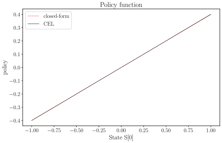
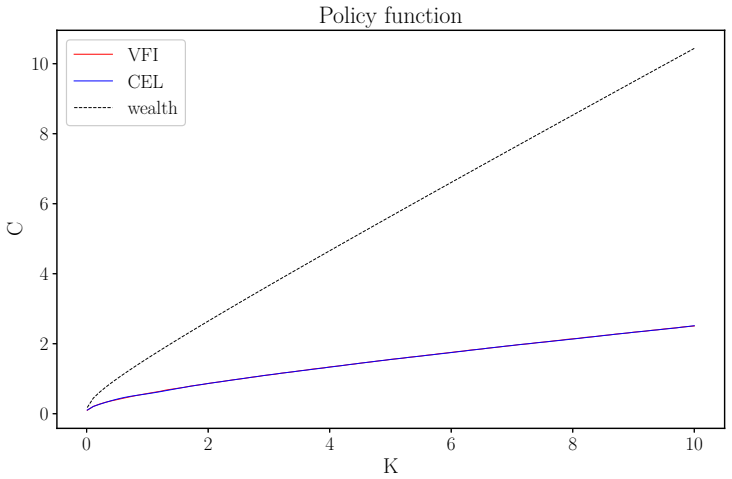
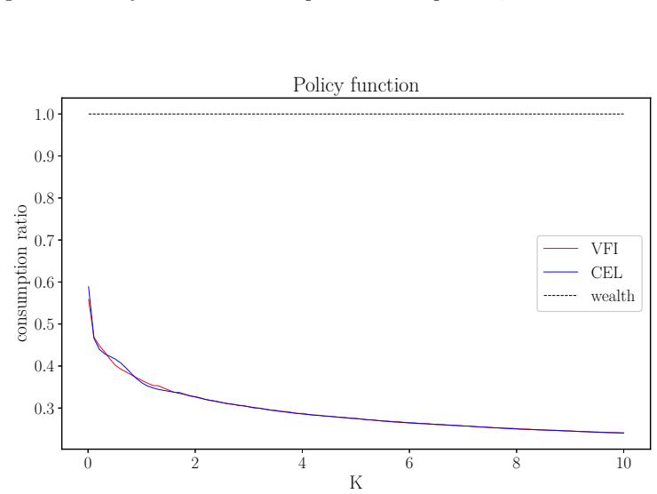
Summary. The paper proposes Certainty Equivalent Learning (CEL), claimed as the first deep-learning algorithm for high-dimensional discrete-time infinite-horizon dynamic programming with recursive utility. CEL represents the value function, policy, and (state-control) certainty-equivalent map by neural networks (three-, four-, or two-network variants), trains them by alternating simulation-based least-squares fitting of the CE operator, policy improvement of the Bellman objective, and value fitting, and stabilizes training with exploratory control noise, Polyak target networks, and delayed policy updates. It requires only forward simulation of the transition and does not use Euler equations, first-order conditions, or differentiability of the law of motion. Expected utility is recovered as a special case. Numerical experiments cover discounted linear-exponential-quadratic-Gaussian control (closed-form, including ns=100, nc=50), small-noise robust control (VFI and closed-form homothetic benchmarks), an Epstein–Zin DSGE with stochastic volatility, and multivariate strategic asset allocation; reported out-of-sample Bellman errors and Euler/FOC residuals typically lie in [1e-4,1e-3].

Significance. If the numerical claims hold, CEL would be a practically useful mesh-free tool for a class of models (Epstein–Zin, risk-sensitive/robust control, long-horizon portfolio choice) that are central in macro-finance yet remain hard for grid-based methods once state or control dimension exceeds a handful of variables. The modular CE-network idea, the explicit comparison with closed-form LEQG and homothetic robust-control solutions, and the out-of-sample residual diagnostics are genuine strengths relative to much of the existing deep-learning DP literature. The careful differentiation from Friedl et al. (2023) and the demonstration that the same framework also covers expected utility further increase potential impact.

major comments (3)

Section 3.1 (third challenge) correctly notes that the plug-in estimator f^{-1}((1/G) sum f(V(s'))) is biased for the true certainty equivalent whenever f^{-1} is nonlinear, with leading bias proportional to (f^{-1})''(M) Var(cM)/2. Yet the training losses for the three- and four-network architectures—Eqs. (28), (32), (44), (49)–(50)—minimize exactly this plug-in residual (or its Ve–D decomposition) with finite G and no bias-correction, importance sampling, or G-scaling study. Target-network Polyak averaging and delayed policy updates stabilize bootstrapping but do not cancel the Jensen bias. Consequently the reported residual band of 1e-4–1e-3 (especially under high curvature: sigma=50/200, gamma=20) does not by itself certify that the learned (V,c,Vc) solve the true Bellman fixed point. A bias audit (e.g., G-refinement, antithetic or control-variate estimators, or a Santos-style residu
The central scalability claim rests on the LEQG experiment with ns=100, nc=50 (Section 4.1.3). While relative value errors <1e-4 and small policy errors are impressive against the closed form, the paper supplies no analogous external benchmark for the non-quadratic applications once dimension rises. In the DSGE (3 states, 2 controls) and multivariate portfolio problems the only diagnostics are internal residuals recomputed by nested Monte Carlo. Without either a high-accuracy reference solution or a quantitative residual-to-welfare/policy-error bound, it remains unclear whether residual levels of 1e-3 translate into economically acceptable approximation error once the CE surface is high-dimensional and strongly curved.
No convergence theory, approximation-rate result, or even a systematic hyper-parameter sensitivity study is provided for the alternating non-convex scheme (Algorithms 3–5). The free parameters (network widths, tau, d, zeta, G, Adam step counts, exploration method) are numerous; the paper’s own discussion of feedback loops between CE learning and policy improvement (Section 3.1, fifth challenge) makes the absence of such analysis material. At minimum, a short ablation on G, tau and the exploration scale, together with multiple random seeds and reported standard errors on the residual tables, is required to support the claim that the method “remains effective in high-dimensional problems.”

minor comments (4)

Abstract and several figure captions contain missing spaces (“accuracycomparabletoVFI”, “out-of-sampleBellmanerrors”). A careful copy-edit pass is needed.
Table 1 and the network-architecture subsections would benefit from an explicit statement of layer widths, activations and output constraints used in each experiment; currently these details are scattered or omitted.
The comparison with Friedl et al. (2023) is thorough, yet the claim “the first deep learning algorithm” should be qualified more carefully in the abstract and introduction once the differences (quadrature vs. learned CE, residual system vs. direct Bellman maximization) have been stated.
Appendix A.2 reports matrices only for the ns=8 case; the high-dimensional LEQG matrices are not supplied, hindering exact replication.

Circularity Check

0 steps flagged

No significant circularity: CEL is an approximate numerical method whose accuracy claims rest on external closed-form/VFI benchmarks and independent out-of-sample residual recomputation, not on tautological restatement of training losses.

full rationale

The paper's derivation chain is a standard simulation-based deep-learning approximation to the Bellman fixed point under recursive utility: neural nets for V, c and Vc (or Ve-D) are trained by alternating minimization of plug-in CE residuals and maximization of the Bellman objective (Eqs. 28-34, 44, 49-52), then evaluated by (i) direct comparison to analytical LEQG and homothetic robust-control solutions, (ii) relative differences versus independent VFI grids, and (iii) out-of-sample Monte-Carlo recomputation of Bellman/Euler/FOC residuals on fresh shocks (Sections 4.1-4.4 and Appendices A.3-A.4). These diagnostics are not the training objectives, use new samples, and are zero only at the true solution; residual size is therefore an independent consistency check rather than a by-construction identity. No parameter is fitted to a data subset and then re-labeled a prediction; no uniqueness theorem or ansatz is imported from the authors' prior work as a load-bearing premise; and the mild self-reference that learned networks are checked against the equations they approximate is ordinary numerical validation, not circularity. The method is therefore self-contained against external anchors.

Axiom & Free-Parameter Ledger

5 free parameters · 5 axioms · 2 invented entities

The paper is a computational-methods contribution. Load-bearing content is the CEL training scheme plus standard recursive-utility DP structure from the literature. Free parameters are training/architecture choices that affect reported accuracy. Axioms are existence of recursive-utility fixed points and the validity of residual diagnostics as accuracy measures. Invented entities are the CEL algorithm and its network decompositions—not physical entities.

free parameters (5)

Neural network widths/depths and activations for V, c, Vc (or Ve, D)
Architecture capacity is chosen by the authors; reported residual levels depend on these choices and are not derived.
Polyak target-update rate τ and policy delay d
Stabilization hyperparameters (Section 3.4) control bootstrap stability; values are design choices, not identified from data.
Exploration scale ζ and Method ∈ {Gaussian, Sobol}
Control-space exploration during simulation (Algorithm 1) is hand-tuned and affects coverage of the state-control domain for CE learning.
Monte Carlo sample sizes N, T, G and optimizer settings (Adam steps Kξ, Kθ, Kϕ, …)
Simulation and training budgets determine residual noise and approximation quality; not fixed by theory.
Model preference/robustness parameters (e.g., σ, γ, β, ψ) in applications
Taken from benchmark calibrations (Hansen–Sargent, Anderson et al., Caldara et al., Campbell et al.); accuracy claims are conditional on these fixed environments.

axioms (5)

domain assumption Recursive utility is well-defined as a fixed point of the Bellman operator with certainty equivalent Vc = f^{-1}(E[f(V(s'))|s,c]) under the stated Markov transition.
Invoked throughout Section 2; existence/uniqueness deferred to cited theory (Hansen–Scheinkman, Stachurski et al., Ma et al.).
ad hoc to paper Neural networks with the chosen architectures can approximate the value, policy, and certainty-equivalent maps to the accuracy needed for residual levels ~1e-4–1e-3.
Implicit universal-approximation reliance; no approximation-rate theorem is proved for the CEL fixed-point iteration.
domain assumption Out-of-sample Bellman errors and Euler/FOC residuals are valid primary accuracy diagnostics for recursive-utility solutions (following Santos 2000-style residual logic).
Section 1 and Section 4 evaluation framework; residuals are necessary but not always sufficient for economic accuracy.
standard math Expected utility is nested when f is linear and the aggregator is additive, so CEL applies to standard expected-utility DP as a special case.
Stated in abstract and Section 2; algebraically standard.
domain assumption State transitions need only be simulable; differentiability of ψ is not required for CEL training.
Methodological premise contrasting Euler-based methods (Introduction; comparison to Friedl et al.).

invented entities (2)

Certainty Equivalent Learning (CEL) algorithm no independent evidence
purpose: Jointly learn value, policy, and certainty-equivalent functions for recursive-utility Bellman equations via alternating simulation-based training.
Core proposed method; validated only by the paper’s own numerical experiments.
Three-/four-/two-network CEL architectures (including Ve − D decomposition of the certainty equivalent) no independent evidence
purpose: Modular functional decompositions of the recursive Bellman equation to stabilize nonlinear CE learning.
Design choices introduced in Section 3.2; usefulness shown only within this paper’s benchmarks.

pith-pipeline@v1.1.0-grok45 · 46625 in / 3913 out tokens · 43830 ms · 2026-07-11T20:25:16.004899+00:00 · methodology

0 comments

read the original abstract

We propose the first deep learning algorithm, the Certainty Equivalent Learning (CEL) algorithm, for solving high-dimensional discrete-time dynamic programming problems with recursive utility. Dynamic programming with recursive utility is numerically challenging because the recursive utility does not have an explicit representation and the Bellman equation contains a certainty equivalent that is difficult to evaluate. The CEL algorithm learns this certainty-equivalent value directly with neural networks and jointly approximates value functions, policy functions, and certainty-equivalent functions. The CEL algorithm is mesh-free and simulation-based, allowing high-dimensional state and control spaces, and does not rely on Euler equations, first-order conditions, or differentiability of the state transition function. The CEL algorithm also works for dynamic programming problems with expected utility as expected utility is a special case of recursive utility. We apply the CEL to discounted linear exponential quadratic Gaussian control, small-noise robust control, Epstein-Zin DSGE, and multivariate strategic asset allocation problems. Compared with closed-form and VFI-based benchmarks, the CEL delivers accurate value and policy approximations, remains effective in high-dimensional problems, achieves accuracy comparable to VFI in the small-noise robust-control case, and produces out-of-sample Bellman errors and Euler or first-order residuals that are in the range from 1.0e-4 to 1.0e-3 for most problems.

Figures

Figures reproduced from arXiv: 2607.04278 by Wu Guo, Xianhua Peng.

**Figure 1.** Figure 1: Value function V (st) comparison for the Gaussian control problem with ns = 8 and nc = 4. The value-function curves are almost indistinguishable across the evaluation domain. In particular, the CEL value function closely matches the closed-form benchmark, indicating that the value network accurately captures the level, curvature, and scale of the true value function. The certainty-equivalent estimates ar… view at source ↗

**Figure 2.** Figure 2: Nested-simulation diagnostic test for the Gaussian benchmark case with [PITH_FULL_IMAGE:figures/full_fig_p039_2.png] view at source ↗

**Figure 3.** Figure 3: Relative error between the CEL value network and the closed-form bench [PITH_FULL_IMAGE:figures/full_fig_p040_3.png] view at source ↗

**Figure 4.** Figure 4: Policy function comparison between the learned CEL policy and the closed [PITH_FULL_IMAGE:figures/full_fig_p041_4.png] view at source ↗

**Figure 5.** Figure 5: Absolute error between the learned CEL policy and the closed-form bench [PITH_FULL_IMAGE:figures/full_fig_p041_5.png] view at source ↗

**Figure 6.** Figure 6: Value function V (st) comparison for the Gaussian control problem with ns = 100 and nc = 50. The value-function curves are closely aligned across the full evaluation range. In particular, the learned CEL value function remains almost indistinguishable from the closed-form benchmark. The certainty-equivalent estimates also stay close to the direct value-network output, suggesting that the certainty-equivale… view at source ↗

**Figure 7.** Figure 7: Nested-simulation diagnostic test for the high-dimensional Gaussian control [PITH_FULL_IMAGE:figures/full_fig_p043_7.png] view at source ↗

**Figure 8.** Figure 8: Relative error between the learned CEL value function and the closed-form [PITH_FULL_IMAGE:figures/full_fig_p044_8.png] view at source ↗

**Figure 9.** Figure 9: Policy function comparison between the learned CEL policy and the closed [PITH_FULL_IMAGE:figures/full_fig_p044_9.png] view at source ↗

**Figure 10.** Figure 10: Absolute error between the learned CEL policy and the closed-form bench [PITH_FULL_IMAGE:figures/full_fig_p045_10.png] view at source ↗

**Figure 11.** Figure 11: Value function and its one-step expansion from the CEL method and VFI [PITH_FULL_IMAGE:figures/full_fig_p048_11.png] view at source ↗

**Figure 12.** Figure 12: Relative difference between the CEL value network and the VFI benchmark [PITH_FULL_IMAGE:figures/full_fig_p048_12.png] view at source ↗

**Figure 13.** Figure 13: Policy function: consumption when capital [PITH_FULL_IMAGE:figures/full_fig_p049_13.png] view at source ↗

**Figure 14.** Figure 14: Policy function: consumption-to-wealth ratio when capital [PITH_FULL_IMAGE:figures/full_fig_p049_14.png] view at source ↗

**Figure 15.** Figure 15: Relative difference between the CEL policy network and the VFI bench [PITH_FULL_IMAGE:figures/full_fig_p050_15.png] view at source ↗

**Figure 16.** Figure 16: Euler residual for the general nonlinear small-noise model with [PITH_FULL_IMAGE:figures/full_fig_p051_16.png] view at source ↗

**Figure 17.** Figure 17: Bellman error for the general nonlinear small-noise model with [PITH_FULL_IMAGE:figures/full_fig_p052_17.png] view at source ↗

**Figure 18.** Figure 18: Value function and its one-step expansion from the CEL method and VFI [PITH_FULL_IMAGE:figures/full_fig_p053_18.png] view at source ↗

**Figure 19.** Figure 19: Relative difference between the CEL value network and the VFI benchmark [PITH_FULL_IMAGE:figures/full_fig_p053_19.png] view at source ↗

**Figure 20.** Figure 20: Policy function: consumption when capital [PITH_FULL_IMAGE:figures/full_fig_p054_20.png] view at source ↗

**Figure 21.** Figure 21: Policy function: consumption-to-wealth ratio when capital [PITH_FULL_IMAGE:figures/full_fig_p054_21.png] view at source ↗

**Figure 22.** Figure 22: Relative difference between the CEL policy network and the VFI bench [PITH_FULL_IMAGE:figures/full_fig_p055_22.png] view at source ↗

**Figure 23.** Figure 23: Euler residual for the general nonlinear small-noise model with [PITH_FULL_IMAGE:figures/full_fig_p056_23.png] view at source ↗

**Figure 24.** Figure 24: Bellman error for the general nonlinear small-noise model with [PITH_FULL_IMAGE:figures/full_fig_p056_24.png] view at source ↗

**Figure 25.** Figure 25: Value function and its one-step expansion from CEL method and VFI [PITH_FULL_IMAGE:figures/full_fig_p058_25.png] view at source ↗

**Figure 26.** Figure 26: Policy function comparison with the analytical solution when [PITH_FULL_IMAGE:figures/full_fig_p059_26.png] view at source ↗

**Figure 27.** Figure 27: Consumption-to-wealth ratio comparison with the analytical solution when [PITH_FULL_IMAGE:figures/full_fig_p059_27.png] view at source ↗

**Figure 28.** Figure 28: Relative error of value function with respect to the analytical solution [PITH_FULL_IMAGE:figures/full_fig_p060_28.png] view at source ↗

**Figure 29.** Figure 29: Relative error of policy function with respect to the analytical solution [PITH_FULL_IMAGE:figures/full_fig_p061_29.png] view at source ↗

**Figure 30.** Figure 30: Value function and its one-step expansion from CEL method and VFI [PITH_FULL_IMAGE:figures/full_fig_p062_30.png] view at source ↗

**Figure 31.** Figure 31: Policy function comparison with the analytical solution when [PITH_FULL_IMAGE:figures/full_fig_p062_31.png] view at source ↗

**Figure 32.** Figure 32: Consumption-to-wealth ratio comparison with the analytical solution when [PITH_FULL_IMAGE:figures/full_fig_p063_32.png] view at source ↗

**Figure 33.** Figure 33: Relative error of value function with respect to the analytical solution [PITH_FULL_IMAGE:figures/full_fig_p064_33.png] view at source ↗

**Figure 34.** Figure 34: Relative error of policy function with respect to the analytical solution [PITH_FULL_IMAGE:figures/full_fig_p064_34.png] view at source ↗

**Figure 35.** Figure 35: Value function comparison for the DSGE model. Capital [PITH_FULL_IMAGE:figures/full_fig_p068_35.png] view at source ↗

**Figure 36.** Figure 36: Policy functions for the DSGE model. The figure reports the consumption [PITH_FULL_IMAGE:figures/full_fig_p068_36.png] view at source ↗

**Figure 37.** Figure 37: Relative Bellman error for the DSGE model. Capital [PITH_FULL_IMAGE:figures/full_fig_p069_37.png] view at source ↗

**Figure 38.** Figure 38: Consumption Euler residual for the DSGE model. Capital [PITH_FULL_IMAGE:figures/full_fig_p070_38.png] view at source ↗

**Figure 39.** Figure 39: Labor FOC residual for the DSGE model. Capital [PITH_FULL_IMAGE:figures/full_fig_p070_39.png] view at source ↗

**Figure 40.** Figure 40: Static condition error for the DSGE model. The condition is derived from [PITH_FULL_IMAGE:figures/full_fig_p071_40.png] view at source ↗

**Figure 41.** Figure 41: Normalized value function for the multivariate strategic asset allocation [PITH_FULL_IMAGE:figures/full_fig_p074_41.png] view at source ↗

**Figure 42.** Figure 42: Consumption-wealth ratio policy function for the multivariate strategic [PITH_FULL_IMAGE:figures/full_fig_p075_42.png] view at source ↗

**Figure 43.** Figure 43: Portfolio-weight policy function for the multivariate strategic asset al [PITH_FULL_IMAGE:figures/full_fig_p076_43.png] view at source ↗

**Figure 44.** Figure 44: Bellman error and static condition error for the multivariate strategic asset [PITH_FULL_IMAGE:figures/full_fig_p077_44.png] view at source ↗

discussion (0)

Reference graph

Works this paper leans on

4 extracted references · 3 linked inside Pith

[1]

M., Xu, Z

Aboussalah, A. M., Xu, Z. and Lee, C.-G. (2022). What is the value of the cross-sectional approach to deep reinforcement learning?,Quantitative Finance 22(6): 1091–1111. Anderson, E. W., Hansen, L. P. and Sargent, T. J. (2012). Small noise methods for risk-sensitive/robust economies,Journal of Economic Dynamics and Control 36(4): 468–500. Andreasen, M. M....

2022
[2]

and Scheidegger, S

Azinovic, M., Gaegauf, L. and Scheidegger, S. (2022). Deep equilibrium nets,Inter- national Economic Review63(4): 1471–1525. Azinovic, M. and Jan Žemlička (2023). Economics-inspired neural networks with stabilizing homotopies,arXiv.Available at https://arxiv.org/abs/2303.14802. Bachouch, A., Huré, C., Langrené, N. and Pham, H. (2022). Deep neural networks...

Pith/arXiv arXiv 2022
[3]

Epstein, L. G. and Zin, S. E. (1989). Substitution, risk aversion, and the temporal behavior of consumption and asset returns: a theoretical framework,Econometrica 57(4): 937–969. Epstein, L. G. and Zin, S. E. (1991). Substitution, risk aversion, and the tempo- ral behavior of consumption and asset returns: An empirical analysis,Journal of political Econo...

Pith/arXiv arXiv 1989
[4]

Kreps, D. M. and Porteus, E. L. (1978). Temporal resolution of uncertainty and dynamic choice theory,Econometrica46(1): 185–200. Lepetyuk, V., Maliar, L. and Maliar, S. (2020). When the US catches a cold, Canada sneezes: A lower-bound tale told by deep learning,Journal of Economic Dynamics and Control117: 103926. Lillicrap, T. P., Hunt, J. J., Pritzel, A....

Pith/arXiv arXiv 1978

[1] [1]

M., Xu, Z

Aboussalah, A. M., Xu, Z. and Lee, C.-G. (2022). What is the value of the cross-sectional approach to deep reinforcement learning?,Quantitative Finance 22(6): 1091–1111. Anderson, E. W., Hansen, L. P. and Sargent, T. J. (2012). Small noise methods for risk-sensitive/robust economies,Journal of Economic Dynamics and Control 36(4): 468–500. Andreasen, M. M....

2022

[2] [2]

and Scheidegger, S

Azinovic, M., Gaegauf, L. and Scheidegger, S. (2022). Deep equilibrium nets,Inter- national Economic Review63(4): 1471–1525. Azinovic, M. and Jan Žemlička (2023). Economics-inspired neural networks with stabilizing homotopies,arXiv.Available at https://arxiv.org/abs/2303.14802. Bachouch, A., Huré, C., Langrené, N. and Pham, H. (2022). Deep neural networks...

Pith/arXiv arXiv 2022

[3] [3]

Epstein, L. G. and Zin, S. E. (1989). Substitution, risk aversion, and the temporal behavior of consumption and asset returns: a theoretical framework,Econometrica 57(4): 937–969. Epstein, L. G. and Zin, S. E. (1991). Substitution, risk aversion, and the tempo- ral behavior of consumption and asset returns: An empirical analysis,Journal of political Econo...

Pith/arXiv arXiv 1989

[4] [4]

Kreps, D. M. and Porteus, E. L. (1978). Temporal resolution of uncertainty and dynamic choice theory,Econometrica46(1): 185–200. Lepetyuk, V., Maliar, L. and Maliar, S. (2020). When the US catches a cold, Canada sneezes: A lower-bound tale told by deep learning,Journal of Economic Dynamics and Control117: 103926. Lillicrap, T. P., Hunt, J. J., Pritzel, A....

Pith/arXiv arXiv 1978