REVIEW 2 major objections 2 minor 2 cited by
Reviewed by Pith at T0; open to challenge.
T0 means a machine referee read the full paper against a public rubric. The mark states how deep the mechanical check went, never who wrote it. the ladder, T0–T4 →
T0 review · grok-4.3
Bistable Memory Recurrent Units enable ultra-low power analog recurrent neural networks via direct parameter-to-circuit mapping and noise suppression at cell boundaries
2026-06-30 22:18 UTC pith:N76ISPAO
load-bearing objection The paper maps BMRUs to current-mode analog circuits with direct parameter correspondence and 20x boundary noise suppression in 180 nm sims, but the first-quadrant fixed-threshold reformulation's effect on expressivity is asserted without shown verification. the 2 major comments →
Hardware-Software Co-Design of Scalable, Energy-Efficient Analog Recurrent Computations
The pith
A machine-rendered reading of the paper's core claim, the machinery that carries it, and where it could break.
Core claim
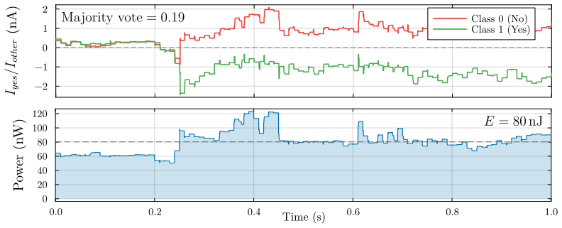
Bistable Memory Recurrent Units admit an ultra-low power current-mode analog implementation which establishes a one-to-one correspondence between each learned parameter and a circuit element; the discrete outputs suppress analog noise by at least 20-fold at each cell boundary, breaking the noise accumulation that prevents analog recurrence. The reformulation for first-quadrant operation with fixed thresholds preserves expressivity and trainability while enabling the direct correspondence.
What carries the argument
Bistable Memory Recurrent Units reformulated for first-quadrant operation with fixed thresholds, which carry the one-to-one parameter-to-circuit-element mapping and enable noise suppression via discrete outputs
Load-bearing premise
Reformulating BMRUs for first-quadrant operation with fixed thresholds preserves expressivity and trainability while enabling direct hardware mapping
What would settle it
A fabricated 180 nm CMOS circuit implementing recurrent BMRUs that shows noise suppression below 20-fold at cell boundaries or deviates from software predictions in recurrent mode would falsify the claim
If this is right
- Power cost of adding recurrence scales linearly with state dimension
- Feedforward layers dominate total power and scale quadratically
- Recurrence is added at linear marginal cost relative to the feedforward backbone
- End-to-end keyword spotting achieves sub-microwatt inference at the RNN core
- Software model serves as high-fidelity low-cost simulator of physical hardware
Where Pith is reading between the lines
- The linear marginal cost of recurrence could allow larger state dimensions in always-on sensors without proportional power growth
- The high-fidelity software simulator could speed iteration on other analog recurrent designs without repeated full transistor simulations
- Sub-microwatt recurrent cores may extend to continuous biomedical monitoring tasks where temporal dynamics matter
- The approach of discrete outputs to break noise accumulation might generalize to other hysteretic or threshold-based analog neural units
Editorial analysis
A structured set of objections, weighed in public.
Referee Report
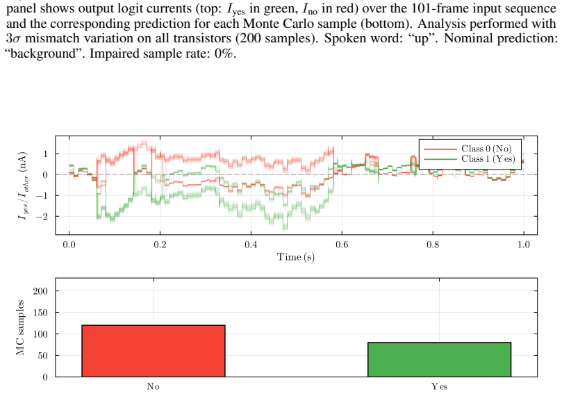
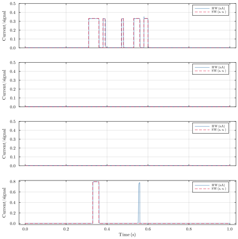
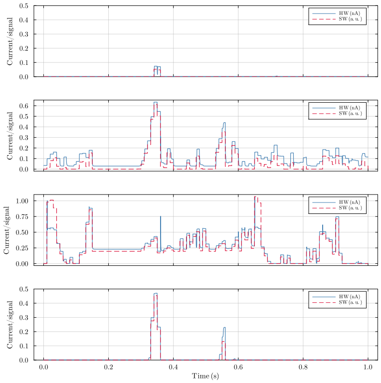
Summary. The paper claims that Bistable Memory Recurrent Units (BMRUs) can be reformulated for first-quadrant current-mode operation with fixed thresholds to enable a direct one-to-one mapping from learned parameters to analog circuit elements in 180 nm CMOS. This mapping, combined with discrete hysteretic outputs, is asserted to suppress analog noise by at least 20-fold at cell boundaries, overcoming noise accumulation in recurrent analog computation. Transistor-level simulations demonstrate near-perfect agreement with the software model, which is then used to show linear marginal power cost for adding recurrence (versus quadratic for feedforward layers) and sub-microwatt end-to-end keyword spotting.
Significance. If the reformulation preserves expressivity and trainability without loss, the result would be significant for always-on edge AI: it supplies a concrete hardware-software co-design path to analog recurrence at ultra-low power, with explicit parameter-to-device correspondence and quantitative noise/power scaling data. The near-perfect simulation fidelity and the reproducible large-scale noise/power analyses are explicit strengths that would allow the software model to serve as a low-cost proxy for hardware exploration.
major comments (2)
- [Abstract and BMRU reformulation section] Abstract and the BMRU reformulation section: the claim that 'reformulation ... with fixed thresholds [preserves] expressivity and trainability' is stated without quantitative support. No comparison is provided of reachable state-transition functions, training convergence, or benchmark accuracy between the original variable-threshold BMRU and the fixed-threshold first-quadrant version. Because the one-to-one parameter-circuit mapping, the 20-fold noise suppression argument, and the linear power-scaling claim all rest on this equivalence, the absence of such verification is load-bearing.
- [Simulation results section] Noise-suppression analysis (simulation results section): the reported 20-fold reduction is obtained from post-reformulation simulations; the text does not derive or bound the suppression factor from the fixed-threshold hysteretic dynamics alone, leaving open whether the factor is an intrinsic property of the reformulated BMRU or an artifact of the particular circuit sizing and input statistics used.
minor comments (2)
- [Circuit design section] Notation for currents and thresholds should be unified between the software model equations and the circuit schematic; inconsistent symbols make the claimed one-to-one correspondence harder to verify by inspection.
- [Application results] The keyword-spotting benchmark description omits the exact RNN topology (number of BMRU layers, hidden dimension) used for the sub-microwatt claim; adding this would allow direct reproduction of the power numbers.
Simulated Author's Rebuttal
We thank the referee for the constructive feedback and for recognizing the potential significance of the BMRU hardware-software co-design. We respond to each major comment below, agreeing that additional quantitative support will strengthen the manuscript.
read point-by-point responses
-
Referee: [Abstract and BMRU reformulation section] Abstract and the BMRU reformulation section: the claim that 'reformulation ... with fixed thresholds [preserves] expressivity and trainability' is stated without quantitative support. No comparison is provided of reachable state-transition functions, training convergence, or benchmark accuracy between the original variable-threshold BMRU and the fixed-threshold first-quadrant version. Because the one-to-one parameter-circuit mapping, the 20-fold noise suppression argument, and the linear power-scaling claim all rest on this equivalence, the absence of such verification is load-bearing.
Authors: We agree that explicit quantitative comparisons are needed to substantiate the preservation of expressivity and trainability under the fixed-threshold reformulation. The reformulation rescales weights and biases to achieve equivalent first-quadrant dynamics while fixing thresholds for circuit mapping. In the revised version we will add a new subsection with side-by-side training convergence curves on standard RNN benchmarks, final test accuracies (including keyword spotting), and a characterization of reachable state-transition functions showing that the fixed-threshold model spans an equivalent functional class via parameter adjustment. revision: yes
-
Referee: [Simulation results section] Noise-suppression analysis (simulation results section): the reported 20-fold reduction is obtained from post-reformulation simulations; the text does not derive or bound the suppression factor from the fixed-threshold hysteretic dynamics alone, leaving open whether the factor is an intrinsic property of the reformulated BMRU or an artifact of the particular circuit sizing and input statistics used.
Authors: The 20-fold suppression is measured in transistor-level simulations of the reformulated circuit. The underlying mechanism is the hysteretic snap to discrete stable points, which quantizes noise at each recurrence step. We acknowledge the manuscript lacks an explicit analytical bound independent of sizing. In revision we will derive a lower bound on the suppression factor from the fixed-threshold dynamics alone: for additive Gaussian noise of std. dev. σ and hysteresis separation Δ, the effective noise variance after the threshold is reduced by a factor of at least Δ/(2σ) with high probability, showing the effect is intrinsic to the bistable dynamics (with the concrete 20× value realized by our chosen Δ/σ ratio). revision: yes
Circularity Check
No significant circularity; derivation relies on independent simulation validation
full rationale
The paper states a reformulation of BMRUs for first-quadrant fixed-threshold operation and asserts that this preserves expressivity and trainability, but provides no equations reducing any claimed performance metric (noise suppression, power scaling, or one-to-one mapping fidelity) directly to fitted parameters or prior results by construction. Transistor-level simulations in 180 nm CMOS are presented as an external check showing agreement with the software model, and power analyses are derived from those simulations rather than tautologically from the reformulation inputs. No load-bearing self-citations, uniqueness theorems, or ansatzes are exhibited in the text that collapse the central claims to their own definitions.
Axiom & Free-Parameter Ledger
axioms (2)
- domain assumption BMRUs constitute a class of RNNs with discrete-valued outputs and hysteretic dynamics that admit direct analog mapping
- ad hoc to paper Reformulation to first-quadrant operation with fixed thresholds preserves expressivity and trainability
read the original abstract
Always-on AI applications, from environmental sensors to biomedical implants, require ultra-low power consumption. Analog circuits offer a path to sub-microwatt inference, yet existing analog implementations are limited to feedforward architectures: extending them to recurrent dynamics has been considered impractical due to noise accumulation through temporal feedback. We demonstrate that this barrier can be overcome through hardware-software co-design. Specifically, we identify that Bistable Memory Recurrent Units (BMRUs), a class of Recurrent Neural Networks (RNNs) with discrete-valued outputs and hysteretic dynamics, admit an ultra-low power current-mode analog implementation which we design from first principles. The resulting circuit establishes a one-to-one correspondence between each learned parameter and a circuit element. The discrete outputs suppress analog noise by at least 20-fold at each cell boundary, breaking the noise accumulation that prevents analog recurrence. We reformulate BMRUs for first-quadrant operation with fixed thresholds, enabling the direct correspondence while preserving expressivity and trainability. Transistor-level simulations in 180 nm Complementary Metal-Oxide-Semiconductor (CMOS) show near-perfect agreement between software predictions and circuit-level behavior, with the software model thereby serving as a high-fidelity simulator of the physical hardware at low computational cost. We leverage this fidelity to conduct large-scale noise immunity and power scaling analyses: the power cost of adding recurrence scales linearly with state dimension, while the feedforward layers dominating total power scale quadratically, meaning recurrence is added at linear marginal cost relative to the feedforward backbone. End-to-end keyword spotting achieves sub-microwatt inference at the RNN core.
Figures


Forward citations
Cited by 2 Pith papers
-
A Fully Tunable Ultra-Low Power Current-Mode Memory Cell in Standard CMOS Technology
A fully tunable ultra-low-power current-mode bistable memory cell using nine standard CMOS transistors enables spike-based logic gates and noise-immune recurrent neural units.
-
A Fully Tunable Ultra-Low Power Current-Mode Memory Cell in Standard CMOS Technology
A nine-transistor current-mode bistable memory cell in 180 nm CMOS is presented with independent tuning of threshold, hysteresis, and gain, shown via schematic simulations for spike-based logic gates and recurrent neu...
Reference graph
Works this paper leans on
-
[1]
LLMCarbon: Modeling the end-to-end carbon footprint of large language models, 2024
Ahmad Faiz, Sotaro Kaneda, Ruhan Wang, Rita Osi, Prateek Sharma, Fan Chen, and Lei Jiang. LLMCarbon: Modeling the end-to-end carbon footprint of large language models, 2024. URL https://arxiv.org/abs/2309.14393
-
[2]
Enrico Barbierato and Alice Gatti. Toward green AI: A methodological survey of the scientific literature.IEEE Access, 12:23989–24013, 2024. doi: 10.1109/ACCESS.2024.3360705
-
[3]
James Kirkpatrick, Razvan Pascanu, Neil Rabinowitz, Joel Veness, Guillaume Desjardins, Andrei A
Mark Horowitz. Computing’s energy problem (and what we can do about it). InIEEE International Solid-State Circuits Conference Digest of Technical Papers, pages 10–14, San Francisco, CA, USA, 2014. IEEE. doi: 10.1109/ISSCC.2014.6757323
-
[4]
Vivienne Sze, Yu-Hsin Chen, Tien-Ju Yang, and Joel S Emer. Efficient processing of deep neural networks: A tutorial and survey.Proceedings of the IEEE, 105(12):2295–2329, 2017. doi: 10.1109/JPROC.2017.2761740
-
[5]
Jihun Lee, Vincent Leung, Ah-Hyoung Lee, Jiannan Huang, Peter Asbeck, Patrick P Mercier, Stephen Shellhammer, Lawrence Larson, Farah Laiwalla, and Arto Nurmikko. Neural record- ing and stimulation using wireless networks of microimplants.Nature Electronics, 4(8): 604–614, 2021. doi: 10.1038/s41928-021-00631-8
-
[6]
Neural Dust: An Ultrasonic, Low Power Solution for Chronic Brain-Machine Interfaces
Dongjin Seo, Jose M Carmena, Jan M Rabaey, Elad Alon, and Michel M Maharbiz. Neural dust: An ultrasonic, low power solution for chronic brain-machine interfaces, 2013. URL https://arxiv.org/abs/1307.2196. 10
work page internal anchor Pith review Pith/arXiv arXiv 2013
-
[7]
Mohammadali Sharifshazileh, Karla Burelo, Johannes Sarnthein, and Giacomo Indiveri. An electronic neuromorphic system for real-time detection of high frequency oscillations (HFO) in intracranial EEG.Nature Communications, 12(1):3095, 2021. doi: 10.1038/ s41467-021-23342-2
work page 2021
-
[8]
Analog versus digital: Extrapolating from electronics to neurobiology
Rahul Sarpeshkar. Analog versus digital: Extrapolating from electronics to neurobiology. Neural Computation, 10(7):1601–1638, 1998. doi: 10.1162/089976698300017052
-
[9]
Memory devices and applications for in-memory computing.Nature Nanotechnology, 15(7): 529–544, 2020
Abu Sebastian, Manuel Le Gallo, Riduan Khaddam-Aljameh, and Evangelos Eleftheriou. Memory devices and applications for in-memory computing.Nature Nanotechnology, 15(7): 529–544, 2020. doi: 10.1038/s41565-020-0655-z
-
[10]
In-memory computing with resistive switching devices
Daniele Ielmini and H-S Philip Wong. In-memory computing with resistive switching devices. Nature Electronics, 1(6):333–343, 2018. doi: 10.1038/s41928-018-0092-2
-
[11]
Ashish Vaswani, Noam Shazeer, Niki Parmar, Jakob Uszkoreit, Llion Jones, Aidan N Gomez, Łukasz Kaiser, and Illia Polosukhin. Attention is all you need. InAdvances in Neural Information Processing Systems, volume 30, Long Beach, CA, USA, 2017
work page 2017
-
[12]
The end of transformers? On challenging attention and the rise of sub-quadratic architectures, 2025
Alexander M Fichtl, Jeremias Bohn, Josefin Kelber, Edoardo Mosca, and Georg Groh. The end of transformers? On challenging attention and the rise of sub-quadratic architectures, 2025. URLhttps://arxiv.org/abs/2510.05364
-
[13]
Efficient transformers: A survey
Yi Tay, Mostafa Dehghani, Dara Bahri, and Donald Metzler. Efficient transformers: A survey. ACM Computing Surveys, 55(6):1–28, 2022. doi: 10.1145/3530811
-
[14]
Efficiently Modeling Long Sequences with Structured State Spaces
Albert Gu, Karan Goel, and Christopher Ré. Efficiently modeling long sequences with structured state spaces, 2022. URLhttps://arxiv.org/abs/2111.00396
work page internal anchor Pith review Pith/arXiv arXiv 2022
-
[15]
Mamba: Linear-time sequence modeling with selective state spaces,
Albert Gu and Tri Dao. Mamba: Linear-time sequence modeling with selective state spaces,
-
[16]
URLhttps://arxiv.org/abs/2312.00752
work page internal anchor Pith review Pith/arXiv arXiv
-
[17]
Tri Dao and Albert Gu. Transformers are SSMs: Generalized models and efficient algorithms through structured state space duality, 2024. URL https://arxiv.org/abs/2405.21060
work page internal anchor Pith review Pith/arXiv arXiv 2024
-
[18]
Linear recurrent units for sequential recommendation
Zhenrui Yue, Yueqi Wang, Zhankui He, Huimin Zeng, Julian McAuley, and Dong Wang. Linear recurrent units for sequential recommendation. InProceedings of the 17th ACM International Conference on Web Search and Data Mining, pages 930–938, Merida, Mexico,
-
[19]
doi: 10.1145/3616855.3635760
-
[20]
The Mamba in the Llama: Distilling and accelerating hybrid models
Junxiong Wang, Daniele Paliotta, Avner May, Alexander Rush, and Tri Dao. The Mamba in the Llama: Distilling and accelerating hybrid models. InAdvances in Neural Information Processing Systems, volume 37, pages 62432–62457, Vancouver, Canada, 2024
work page 2024
-
[21]
On the parameterization and initialization of diagonal state space models
Albert Gu, Ankit Gupta, Karan Goel, and Christopher Ré. On the parameterization and initialization of diagonal state space models. InAdvances in Neural Information Processing Systems, volume 35, pages 35971–35983, New Orleans, LA, USA, 2022
work page 2022
-
[22]
Stephen Boyd and Leon Chua. Fading memory and the problem of approximating nonlinear operators with Volterra series.IEEE Transactions on Circuits and Systems, 32(11):1150–1161,
-
[23]
doi: 10.1109/TCS.1985.1085649
-
[24]
A bio-inspired bistable recurrent cell allows for long-lasting memory.PLOS ONE, 16(6):e0252676, 2021
Nicolas Vecoven, Damien Ernst, and Guillaume Drion. A bio-inspired bistable recurrent cell allows for long-lasting memory.PLOS ONE, 16(6):e0252676, 2021. doi: 10.1371/journal. pone.0252676
-
[25]
Gaspard Lambrechts, Florent De Geeter, Nicolas Vecoven, Damien Ernst, and Guillaume Drion. Warming up recurrent neural networks to maximise reachable multistability greatly improves learning.Neural Networks, 166:645–669, 2023. doi: 10.1016/j.neunet.2023.07.023
-
[26]
Eve Marder, L F Abbott, Gina G Turrigiano, Zhengyu Liu, and Jorge Golowasch. Memory from the dynamics of intrinsic membrane currents.Proceedings of the National Academy of Sciences, 93(24):13481–13486, 1996. doi: 10.1073/pnas.93.24.13481. 11
-
[27]
Neural Computation 9, 1735–1780
Sepp Hochreiter and Jürgen Schmidhuber. Long short-term memory.Neural Computation, 9 (8):1735–1780, 1997. doi: 10.1162/neco.1997.9.8.1735
-
[28]
Learning phrase representations using RNN encoder- decoder for statistical machine translation, 2014
Kyunghyun Cho, Bart Van Merriënboer, Caglar Gulcehre, Dzmitry Bahdanau, Fethi Bougares, Holger Schwenk, and Yoshua Bengio. Learning phrase representations using RNN encoder- decoder for statistical machine translation, 2014. URL https://arxiv.org/abs/1406. 1078
work page 2014
-
[29]
Yoshua Bengio, Patrice Simard, and Paolo Frasconi. Learning long-term dependencies with gradient descent is difficult.IEEE Transactions on Neural Networks, 5(2):157–166, 1994. doi: 10.1109/72.279181
-
[30]
On the difficulty of training recurrent neural networks
Razvan Pascanu, Tomas Mikolov, and Yoshua Bengio. On the difficulty of training recurrent neural networks. InInternational Conference on Machine Learning, pages 1310–1318, Atlanta, GA, USA, 2013. PMLR
work page 2013
-
[31]
Raju Machupalli, Masum Hossain, and Mrinal Mandal. Review of ASIC accelerators for deep neural network.Microprocessors and Microsystems, 89:104441, 2022. doi: 10.1016/j.micpro. 2022.104441
-
[32]
Yu-Hsin Chen, Tien-Ju Yang, Joel Emer, and Vivienne Sze. Eyeriss v2: A flexible accelerator for emerging deep neural networks on mobile devices.IEEE Journal on Emerging and Selected Topics in Circuits and Systems, 9(2):292–308, 2019. doi: 10.1109/JETCAS.2019.2910232
-
[33]
Soroush Heydari and Qusay H Mahmoud. Tiny machine learning and on-device inference: A survey of applications, challenges, and future directions.Sensors, 25(10):3191, 2025. doi: 10.3390/s25103191
-
[34]
Colby Banbury, Vijay Janapa Reddi, Peter Torelli, Jeremy Holleman, Nat Jeffries, Csaba Kiraly, Pietro Montino, David Kanter, Sebastian Ahmed, Danilo Pau, et al. MLPerf tiny benchmark, 2021. URLhttps://arxiv.org/abs/2106.07597
work page Pith review arXiv 2021
-
[35]
Pete Warden and Daniel Situnayake.TinyML: Machine Learning with TensorFlow Lite on Arduino and Ultra-Low-Power Microcontrollers. O’Reilly Media, 2019
work page 2019
-
[36]
MCUNet: Tiny deep learning on IoT devices
Ji Lin, Wei-Ming Chen, Yujun Lin, John Cohn, Chuang Gan, and Song Han. MCUNet: Tiny deep learning on IoT devices. InAdvances in Neural Information Processing Systems, volume 33, pages 11711–11722, Virtual, 2020
work page 2020
-
[37]
SpArSe: Sparse architecture search for CNNs on resource-constrained microcontrollers
Igor Fedorov, Ryan P Adams, Matthew Mattina, and Paul N Whatmough. SpArSe: Sparse architecture search for CNNs on resource-constrained microcontrollers. InAdvances in Neural Information Processing Systems, volume 32, Vancouver, Canada, 2019
work page 2019
-
[38]
Wolfgang Maass, Thomas Natschläger, and Henry Markram. Real-time computing without stable states: A new framework for neural computation based on perturbations.Neural Computation, 14(11):2531–2560, 2002. doi: 10.1162/089976602760407955
-
[39]
Loihi: A neuromorphic manycore processor with on-chip learning.IEEE Micro, 38(1):82–99, 2018
Mike Davies, Narayan Srinivasa, Tsung-Han Lin, Gautham Chinya, Yongqiang Cao, Sri Harsha Choday, Georgios Dimou, Prasad Joshi, Nabil Imam, Shweta Jain, et al. Loihi: A neuromorphic manycore processor with on-chip learning.IEEE Micro, 38(1):82–99, 2018. doi: 10.1109/ MM.2018.112130359
-
[40]
Efficient neuromorphic signal processing with Loihi 2
Garrick Orchard, E Paxon Frady, Daniel Ben Dayan Rubin, Sophia Sanborn, Sumit Bam Shrestha, Friedrich T Sommer, and Mike Davies. Efficient neuromorphic signal processing with Loihi 2. InIEEE Workshop on Signal Processing Systems (SiPS), pages 254–259, Coimbra, Portugal, 2021. IEEE. doi: 10.1109/SiPS52927.2021.00053
-
[41]
Neuromorphic electronic systems.Proceedings of the IEEE, 78(10):1629–1636,
Carver Mead. Neuromorphic electronic systems.Proceedings of the IEEE, 78(10):1629–1636,
-
[42]
doi: 10.1109/5.58356
-
[43]
Memristive crossbar arrays for brain-inspired computing
Qiangfei Xia and J Joshua Yang. Memristive crossbar arrays for brain-inspired computing. Nature Materials, 18(4):309–323, 2019. doi: 10.1038/s41563-019-0291-x. 12
-
[44]
Mirko Prezioso, Farnood Merrikh-Bayat, Brian D Hoskins, Gina C Adam, Konstantin K Likharev, and Dmitri B Strukov. Training and operation of an integrated neuromorphic network based on metal-oxide memristors.Nature, 521(7550):61–64, 2015. doi: 10.1038/nature14441
-
[45]
Mostafa Rahimi Azghadi, Corey Lammie, Jason K Eshraghian, Melika Payvand, Elisa Donati, Bernabe Linares-Barranco, and Giacomo Indiveri. Hardware implementation of deep network accelerators towards healthcare and biomedical applications.IEEE Transactions on Biomedical Circuits and Systems, 14(6):1138–1159, 2020. doi: 10.1109/TBCAS.2020.3036081
-
[46]
Can Li, Miao Hu, Yunning Li, Hao Jiang, Ning Ge, Eric Montgomery, Jiaming Zhang, Wenhao Song, Noraica Dávila, Catherine E Graves, et al. Long short-term memory networks in memristor crossbar arrays.Nature Machine Intelligence, 1(1):49–57, 2019. doi: 10.1038/ s42256-018-0001-4
work page 2019
-
[47]
A review of computing with spiking neural networks.Computers, Materials & Continua, 78(3):2909, 2024
Jiadong Wu, Yinan Wang, Zhiwei Li, Lun Lu, and Qingjiang Li. A review of computing with spiking neural networks.Computers, Materials & Continua, 78(3):2909, 2024. doi: 10.32604/cmc.2024.047240
-
[48]
Towards spike-based machine intelligence with neuromorphic computing.Nature, 575(7784):607–617, 2019
Kaushik Roy, Akhilesh Jaiswal, and Priyadarshini Panda. Towards spike-based machine intelligence with neuromorphic computing.Nature, 575(7784):607–617, 2019. doi: 10.1038/ s41586-019-1677-2
work page 2019
-
[49]
Nicholas LeBow, Bodo Rueckauer, Pengfei Sun, Meritxell Rovira, Cecilia Jiménez-Jorquera, Shih-Chii Liu, and Josep Maria Margarit-Taulé. Real-time edge neuromorphic tasting from chemical microsensor arrays.Frontiers in Neuroscience, 15:771480, 2021. doi: 10.3389/fnins. 2021.771480
-
[50]
Catherine D Schuman, Shruti R Kulkarni, Maryam Parsa, J Parker Mitchell, Bill Kay, and Prasanna Date. Opportunities for neuromorphic computing algorithms and applications.Nature Computational Science, 2(1):10–19, 2022. doi: 10.1038/s43588-021-00184-y
-
[51]
Recurrent Neural Networks Hardware Implementation on FPGA
Andre Xian Ming Chang, Berin Martini, and Eugenio Culurciello. Recurrent neural networks hardware implementation on FPGA, 2015. URLhttps://arxiv.org/abs/1511.05552
work page internal anchor Pith review Pith/arXiv arXiv 2015
-
[52]
Nadezhda Semenova and Daniel Brunner. Noise-mitigation strategies in physical feedforward neural networks.Chaos: An Interdisciplinary Journal of Nonlinear Science, 32(6):061106,
-
[53]
doi: 10.1063/5.0096637
-
[54]
Jack Kendall, Ross Pantone, Kalpana Manickavasagam, Yoshua Bengio, and Benjamin Scellier. Training end-to-end analog neural networks with equilibrium propagation, 2020. URL https: //arxiv.org/abs/2006.01981
- [55]
-
[56]
AML100 - near-zero power analogml processor
Aspinity. AML100 - near-zero power analogml processor. https://www.aspinity.com/ aml100, 2022. Product information page, accessed: 2026-05-05
work page 2022
-
[57]
NDP120 neural decision processor
Syntiant. NDP120 neural decision processor. https://www.syntiant.com/s/ Syntiant-Product_Brief_NDP120.pdf, 2021. Product brief, accessed: 2026-05-05
work page 2021
-
[58]
Parallelizable memory recurrent units
Florent De Geeter, Gaspard Lambrechts, Damien Ernst, and Guillaume Drion. Parallelizable memory recurrent units, 2026. URLhttps://arxiv.org/abs/2601.09495
work page internal anchor Pith review Pith/arXiv arXiv 2026
-
[59]
Pararnn: Unlocking parallel training of nonlinear rnns for large language models, 2025
Federico Danieli, Pau Rodríguez, Miguel Sarabia, Xavier Suau, and Luca Zappella. ParaRNN: Unlocking parallel training of nonlinear RNNs for large language models, 2025. URL https: //arxiv.org/abs/2510.21450
-
[60]
Parallelizing linear recurrent neural nets over sequence length,
Eric Martin and Chris Cundy. Parallelizing linear recurrent neural nets over sequence length,
-
[61]
URLhttps://arxiv.org/abs/1709.04057
work page internal anchor Pith review Pith/arXiv arXiv
-
[62]
Speech Commands: A Dataset for Limited-Vocabulary Speech Recognition
Pete Warden. Speech commands: A dataset for limited-vocabulary speech recognition, 2018. URLhttps://arxiv.org/abs/1804.03209. 13
work page internal anchor Pith review Pith/arXiv arXiv 2018
-
[63]
Resurrecting recurrent neural networks for long sequences, 2023
Antonio Orvieto, Samuel L Smith, Albert Gu, Anushan Fernando, Caglar Gulcehre, Razvan Pascanu, and Soham De. Resurrecting recurrent neural networks for long sequences, 2023. URLhttps://arxiv.org/abs/2303.06349
-
[64]
Leo Feng, Frederick Tung, Mohamed Osama Ahmed, Yoshua Bengio, and Hossein Hajimir- sadeghi. Were RNNs all we needed?, 2024. URLhttps://arxiv.org/abs/2410.01201
-
[65]
On the Importance of Multistability for Horizon Generalization in Reinforcement Learning
Asad Bakija, Florent De Geeter, Julien Brandoit, Pierre Sacré, and Guillaume Drion. On the importance of multistability for horizon generalization in reinforcement learning, 2026. URL https://arxiv.org/abs/2605.12206
work page internal anchor Pith review Pith/arXiv arXiv 2026
-
[66]
Matching properties of MOS transistors.IEEE Journal of Solid-State Circuits, 24(5):1433–1439, 1989
Marcel J M Pelgrom, Aad C J Duinmaijer, and Anton P G Welbers. Matching properties of MOS transistors.IEEE Journal of Solid-State Circuits, 24(5):1433–1439, 1989. doi: 10.1109/JSSC.1989.572629
-
[67]
Peter R Kinget. Device mismatch and tradeoffs in the design of analog circuits.IEEE Journal of Solid-State Circuits, 40(6):1212–1224, 2005. doi: 10.1109/JSSC.2005.848021
-
[68]
Mohtashim Mansoor, Ibraheem Haneef, Suhail Akhtar, Andrea De Luca, and Florin Udrea. Silicon diode temperature sensors—a review of applications.Sensors and Actuators A: Physical, 232:63–74, 2015. doi: 10.1016/j.sna.2015.04.022
-
[69]
Long range arena: A benchmark for efficient transformers.arXiv preprint arXiv:2011.04006,
Yi Tay, Mostafa Dehghani, Samira Abnar, Yikang Shen, Dara Bahri, Philip Pham, Jinfeng Rao, Liu Yang, Sebastian Ruder, and Donald Metzler. Long range arena: A benchmark for efficient transformers, 2021. URLhttps://arxiv.org/abs/2011.04006
-
[70]
Andrej Karpathy. nanoGPT, 2022. URL https://github.com/karpathy/nanoGPT. GitHub repository
work page 2022
-
[71]
Digital twin: Enabling technologies, challenges and open research.IEEE Access, 8:108952–108971, 2020
Iván López-Espejo, Zheng-Hua Tan, John H L Hansen, and Jesper Jensen. Deep spoken keyword spotting: An overview.IEEE Access, 10:4169–4199, 2022. doi: 10.1109/ACCESS. 2021.3139508
-
[72]
Geoffrey Hinton, Li Deng, Dong Yu, George E Dahl, Abdel-rahman Mohamed, Navdeep Jaitly, Andrew Senior, Vincent Vanhoucke, Patrick Nguyen, Tara N Sainath, et al. Deep neural networks for acoustic modeling in speech recognition: The shared views of four research groups.IEEE Signal Processing Magazine, 29(6):82–97, 2012. doi: 10.1109/MSP.2012. 2205597
-
[73]
Small-footprint keyword spotting using deep neural networks
Guoguo Chen, Carolina Parada, and Georg Heigold. Small-footprint keyword spotting using deep neural networks. InIEEE International Conference on Acoustics, Speech and Signal Processing (ICASSP), pages 4087–4091, Florence, Italy, 2014. IEEE. doi: 10.1109/ICASSP. 2014.6854370
-
[74]
Convolutional Recurrent Neural Networks for Small-Footprint Keyword Spotting
Sercan O Arik, Markus Kliegl, Rewon Child, Joel Hestness, Andrew Gibiansky, Chris Fougner, Ryan Prenger, and Adam Coates. Convolutional recurrent neural networks for small-footprint keyword spotting, 2017. URLhttps://arxiv.org/abs/1703.05390
work page internal anchor Pith review Pith/arXiv arXiv 2017
-
[75]
Steven Davis and Paul Mermelstein. Comparison of parametric representations for monosyl- labic word recognition in continuously spoken sentences.IEEE Transactions on Acoustics, Speech, and Signal Processing, 28(4):357–366, 1980. doi: 10.1109/TASSP.1980.1163420
-
[76]
Daniel Augusto Villamizar, Dante Gabriel Muratore, James B Wieser, and Boris Murmann. An 800 nW switched-capacitor feature extraction filterbank for sound classification.IEEE Transactions on Circuits and Systems I: Regular Papers, 68(4):1578–1588, 2021. doi: 10. 1109/tcsi.2020.3047035
-
[77]
Heejin Yang, Ji-Hwan Seol, Rohit Rothe, Zichen Fan, Qirui Zhang, Hun-Seok Kim, David Blaauw, and Dennis Sylvester. A 1.5- µw fully-integrated keyword spotting SoC in 28-nm CMOS with skip-RNN and fast-settling analog frontend for adaptive frame skipping.IEEE Journal of Solid-State Circuits, 59(1):29–39, 2023. doi: 10.1109/jssc.2023.3316648
-
[78]
Cadence Design Systems. Cadence Virtuoso Platform. https://www.cadence.com/en_ US/home/tools/custom-ic-analog-rf-design/virtuoso-studio.html, 2023. 14
work page 2023
-
[79]
Oxford University Press, 3rd edition, 2011
Phillip E Allen and Douglas R Holberg.CMOS Analog Circuit Design. Oxford University Press, 3rd edition, 2011
work page 2011
-
[80]
Behzad Razavi.Design of Analog CMOS Integrated Circuits. McGraw-Hill, 2001
work page 2001
discussion (0)
Sign in with ORCID, Apple, or X to comment. Anyone can read and Pith papers without signing in.