REVIEW 5 major objections 4 minor 2 cited by
Multi-modal contrastive learning adapts to intrinsic dimensions of shared latent variables
T0 review · 5 major / 4 minor · reviewed 2026-08-15 · deepseek-v4-flash
Pith's one-line read Multi-modal contrastive learning with optimized temperature provably selects representations whose intrinsic dimension equals that of the shared latent variables, independent of the specified output dimension.
desk verdict A genuinely new theory of temperature-optimized InfoNCE, but the intrinsic-dimension claim leans on an unverified existence assumption that the paper only supports with indirect evidence. read the letter →
The pith
A machine-rendered reading of the paper's core claim, the machinery that carries it, and where it could break.
The reading
What carries the argument
The load-bearing identity is the variational decomposition of the infoNCE loss (Lemma 8): $L(f,g,\tau)+2I(f(X);g(Y)) = D_{\mathrm{KL}}(P_{f(X),g(Y)}\|Q_{f(X),g(Y),\tau}) + D_{\mathrm{KL}}(P_{f(X),g(Y)}\|\tilde Q_{f(X),g(Y),\tau})$, where the two auxiliary distributions are kernel-smoothed versions of the joint law. Discretizing the bounded normalized representations onto nested partitions makes every mutual information finite and turns maximal mutual information into a well-defined order $W(H)$; near-minimizers are defined as $O_{L,\eta}(H)$ with a temperature floor $\varepsilon(\eta)\to0$. The set $V(H)=A(H)\cap W(H)$ bundles alignment (normalized equality plus similarity at its essential supremum) with maximal discretized mutual information, and Proposition 1 gives all such ideal pairs a common intrinsic dimension $k^*$. The proof then shows minimizers cannot exceed $k^*$ (using conditional expectation and Jensen to build a strictly better representation unless $f,g$ factor through $f^*,g^*$) and cannot fall below it (using data processing to boost mutual information).
What would settle it
Train the InfoNCE objective with optimized temperature on synthetic data with a known shared latent dimension, as in Section 1.1, and measure the intrinsic dimension of the learned representations and the temperature trajectory. If the estimated intrinsic dimension tracks the user-specified output dimension $d$ instead of stabilizing at $k^*$, or if $\tau$ does not converge to zero, Theorem 2's prediction fails; the paper's own two-layer ReLU example with $A(H)=\varnothing$ already shows the kind of degeneracy that would appear.
Extended reading notes
Core claim
On the population InfoNCE loss $L(f,g,\tau)$ with normalized inner-product similarity, and assuming $V(H)=A(H)\cap W(H)\neq\varnothing$ and $H$ contains all measurable functions, Theorem 2 characterizes the minimizer set $\bigcap_{\eta\ge0}O_{L,\eta}(H)$. Every pair $(f,g)$ in this set satisfies: (1) $\sigma(f(X),g(Y))=m_\sigma(f,g)$ almost surely, so positive-pair similarity reaches its essential supremum; (2) $ID(f)=ID(g)=k^*$, where $k^*$ is the common intrinsic dimension of ideal aligned representations and $ID(\cdot)$ is defined through factorization $f=\phi\circ h$ with $\dim(R(h))=k$ and $\phi$ injective; (3) the infoNCE loss $L(f,g,\tau)$ is increasing in $\tau$; and (4) $(f,g)\in W(H)$ in the fine-grained discretized mutual-information order. The paper reads these as the reason the optimized temperature collapses to zero in practice and why out-of-sample matching accuracy and estimated intrinsic dimension saturate once the output dimension exceeds $k^*$.
Load-bearing premise
The argument assumes that at least one pair of encoder functions is both perfectly aligned (normalized outputs equal almost surely with similarity at its maximum) and achieves the best possible discretized mutual information; the paper assumes this condition $V(H)\neq\varnothing$ rather than proving it for neural network classes.
Editorial extensions
If this is right
- For any user-specified output dimension $d\ge k^*$, the learned representation essentially lives on a $k^*$-dimensional manifold, so downstream matching or classification accuracy should saturate once $d\ge k^*$.
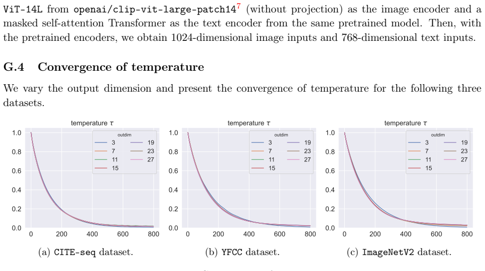
- Optimizing temperature is not a hyperparameter detail: it is what forces dimension adaptation, and the theory predicts $\tau\to0^+$ along training.
- A two-stage fitting strategy is suggested: train with a large output dimension for expressiveness, then project the learned representation onto its discovered intrinsic dimension to speed up inference.
- When the output dimension is correctly specified as $k^*$, the minimizer set coincides with aligned, uniform, mutual-information-maximizing representations (Theorem 3 in Appendix E.2).
- Under an additional condition, the learned representations are sufficient in the dimension-reduction sense $Y \perp\!\!\perp X \mid f^*(X)$ (Proposition 2), connecting CLIP to sufficient dimension reduction.
Reading between the lines
- We infer that the theory supplies a practical diagnostic: fit the contrastive objective at several output dimensions and estimate the intrinsic dimension of the learned embeddings; the plateau value is a label-free estimate of $k^*$.
- We infer that in finite samples the temperature need not literally vanish; the testable prediction is that its training path tends to zero, so monitoring $\tau$ is a cheap check of whether the function class is expressive enough for the assumption $V(H)\neq\varnothing$.
- We infer that the same mechanism should extend to other contrastive losses that admit a variational mutual-information bound plus KL penalties with a tunable scale parameter, producing analogous collapse onto the shared latent subspace.
- We infer that when each modality has its own intrinsic dimension, the theorem predicts each encoder separately collapses to the common shared dimension $k^*$, a property that could be tested by cross-modal retrieval accuracy and per-modality reconstruction quality.
Signed reviews
Editorial analysis
A structured set of objections, weighed in public.
Referee Report
Summary. The paper studies the population InfoNCE loss for multimodal contrastive learning (CLIP-style training) with temperature optimization, beyond linear models and specific distributions. It introduces two properties of ideal representations—alignment/similarity maximization (A(H)) and maximal discretized mutual information (W(H))—and defines V(H) as their intersection. Under the assumption V(H)≠∅ and a function class containing all measurable functions, Theorem 2 claims that every approximate minimizer (f,g) in ∩_{η≥0}O_{L,η}(H) satisfies: (1) σ(f(X),g(Y)) equals its essential supremum almost surely; (2) ID(f)=ID(g)=k*, the intrinsic dimension of the shared latent variables; (3) the InfoNCE loss is increasing in temperature; and (4) (f,g) maximizes mutual information. The paper also connects the result to sufficient dimension reduction and reports experiments on synthetic data, CITE-seq, ImageNetV2, and YFCC showing saturation of downstream accuracy and estimated intrinsic dimension, plus temperature decay.
Significance. If the main theorem is correct under its stated assumptions, the paper makes a substantive contribution: it gives a precise sense in which temperature optimization in InfoNCE can select representations of exactly the intrinsic dimension of the shared latent variables, without requiring the uniform-on-the-hypersphere assumption of Wang and Isola (2020). The variational decomposition in Lemma 8, the discretization framework, and the connection to sufficient dimension reduction are useful conceptual tools. The paper also ships falsifiable predictions—similarity concentration, temperature decay, and saturation of estimated intrinsic dimension—and verifies them in several experiments. These are genuine strengths. The main weakness is that the central result is conditional on V(H)≠∅, which is not established for the neural-network classes used in the experiments, and the formal theorem statement omits the universal-function-class condition that the proof actually uses.
major comments (5)
- [Section 2.1, Definition 1; Appendix B, Definition 4; Appendix C.2.1] The definition of A(H) in the main text omits the condition mσ(f,g)=1 that appears in the appendix version and in Table 1. This is not a harmless typo: the proof of Lemma 9 in Appendix C.2.1 uses the stronger statement '(f*,g*)∈A(H), i.e., f*(X)=g*(Y) almost surely' and then evaluates the KL divergence with an exponent e^{1/τ} on the diagonal. These steps require pointwise unit norms of the normalized representations and mσ=1, neither of which follows from Definition 1 as printed. Because V(H)=A(H)∩W(H) is the central premise of Theorem 2, please reconcile the two definitions and re-check Lemma 9 and Lemma 10 under the corrected definition.
- [Section 3.2, Theorem 2 and proof in Appendix D.2] The formal statement of Theorem 2 says only 'Assume V(H)≠∅', but the proof requires H to contain all measurable functions. In Step 2 (Appendix D.2) the map f*(X)=E[f(X)|f*(X)] is used as an element of H_X, and Lemma 7(2) (Appendix B.2) constructs arbitrary measurable functions Φ1,Φ2 to force a strict mutual-information gain. These steps do not go through for the 5-layer ReLU classes used in Section 4. Please add the universal-function-class assumption to the theorem statement, or prove the result for the actual function classes; as stated, the theorem is stronger than what is proved.
- [Section 2.1, V(H)≠∅; Appendix G.2; Appendix G.4] The central dimension-adaptation conclusion is conditional on V(H)≠∅, and for neural-network function classes this is assumed rather than established. The paper's own Appendix G.2 shows that when A(H)=∅ in a 2-layer ReLU class, minimizers can have mσ=0 and the similarity-maximization conclusion of Theorem 2 fails. The only empirical evidence offered for V(H)≠∅ in the 5-layer ReLU class is temperature decay in Appendix G.4, which is consistent with many other mechanisms. Without a verification—or at least a characterization—of V(H) for the architectures used in the experiments, the claim that CLIP adapts to intrinsic dimension for these networks is not supported by the theorem.
- [Appendix C.2.2, proof of Lemma 10(1)(2)] The proof invokes the Moore-Osgood theorem to interchange the limits in j and M, concluding limsup_M Δ_M(0)=0 and liminf_M(I_M−I*_M)=0 from the chain of inequalities limsup_M{I*_M−I_M+Δ_M(τ_j)}≤η_j. Moore-Osgood requires conditions such as uniform convergence or monotonicity in one of the limits, and here the quantities are limsups/liminfs rather than ordinary limits; no such conditions are verified. Since this step underlies Theorem 2(1) and (4), please supply a rigorous justification or replace the argument.
- [Appendix C.2.1, proof of Lemma 9] The proof that C* is nonempty claims the constant function ω(η)=0 is in C*, but for η=0 this requires a pair (f,g) and τ≥0 with limsup_M(L(f_M,g_M,τ)+2I*_M(H))≤0. The displayed argument only establishes convergence to 0 as τ→0+, not attainment at some τ≥0. The definition of ε(η) in Eq. (9) and the nonemptiness of ∩_{η≥0}O_{L,η}(H) therefore need a more careful construction, for example an explicit rate ω(η)>0 with ω(η)→0.
minor comments (4)
- [Section 2.2, Definition 3] The phrase 'almost everywhere' in Definition 3 should specify the measure; later proofs use 'almost surely' under the law of (X,Y) interchangeably. Please clarify whether equality is required almost everywhere with respect to Lebesgue measure or almost surely under the data distribution.
- [Appendix D.1, Step 1] The notation Z∈B^k is used without defining B^k; it should presumably be eB^k or R^k.
- [Appendix G.2] The sentence 'the intrinsic dimension k*=2 is correctly specified' in the V(H)=∅ example appears to conflict with the paper's claim that dimension adaptation and similarity maximization are jointly delivered by Theorem 2; please clarify what remains true outside V(H).
- [Eq. (3) and Eq. (9)] The definition of O_{L,η}(H) in Eq. (3) uses ε(η) before ε(·) is formally introduced in Eq. (9); please reorder the presentation or add a forward reference.
Circularity Check
Theorem 2(4) largely restates the benchmark built into the minimizer definition; the dimension-adaptation claim itself is derived, not fitted.
-
self definitional
[Section 3.1 Eq. (3); Section 2.1 Definition 2; Theorem 2(4)]
"O_{L,η}(H) = {(f,g)∈H : ∃τ≥ε(η), lim sup_{M→+∞}(L(f_M,g_M,τ)+2I^*_M(H)) ≤ 2η} ... W(H) = {(f,g)∈H : lim inf_{M→+∞}(I(f_M(X);g_M(Y))−I^*_M(H)) ≥ 0} ... (mutual information maximization) (f,g)∈W(H)."
Lemma 8 gives L(f_M,g_M,τ)+2I^*_M(H) = 2(I^*_M(H)−I(f_M;g_M)) + 2Δ(P;Q,Q~) with Δ≥0. Therefore membership in ∩_{η≥0}O_{L,η}(H) forces limsup_M(I^*_M(H)−I(f_M;g_M))≤0, i.e. liminf_M(I(f_M;g_M)−I^*_M(H))≥0, which is exactly the inequality defining W(H). So Theorem 2(4) is the near-minimizer criterion (3) unpacked, not an independent prediction obtained from minimizing the raw InfoNCE loss; the benchmark I^*_M(H) is already part of the definition of the solution set. The dimension-adaptation conclusion (Theorem 2(2)) is separate and is genuinely derived via Lemma 7 and the two-step argument.
full rationale
The paper's central dimension-adaptation theorem does not fit any parameter to its conclusion and does not rely on a self-citation chain: it follows from the variational decomposition (Lemma 8), the near-minimizer set (3), and the sufficiency property of V(H) (Lemma 7). The one definitional reduction is Theorem 2(4): because both the minimizer set and W(H) are defined through I^*_M(H), the mutual-information-maximization conclusion restates the benchmark used to define O_{L,η}(H). This is a formalization artifact rather than a fitted prediction, and it leaves the intrinsic-dimension and temperature-monotonicity results with independent mathematical content. The main caveat is not circularity but scope: the theorem is conditional on V(H)≠∅, which the paper assumes (Section 2.1) and only indirectly supports by temperature decay (Appendix G.4); Appendix G.2 shows degeneracies (m_σ=0) when V(H)=∅. Under the hard rules, an unverified assumption is a correctness/robustness concern, not circularity. Overall score reflects one secondary conclusion that reduces by construction while the central claim stands independently: 4.
Assumptions & free parameters
assumptions (5)
- domain assumption V(H) is nonempty: there exist aligned representations (normalized equality and maximal similarity) that also achieve maximal discretized mutual information over the function class.
- domain assumption H includes all measurable functions of X and Y.
- standard math Standard measure-theoretic regularity: representations have compact range, densities exist, and discretization limits converge as in Lemmas 1 to 5.
- domain assumption The similarity measure is the population-normalized inner product and ideal representations reach m_sigma = 1.
- ad hoc to paper In experiments, the Levina-Bickel MLE estimator approximates the intrinsic dimension ID(f).
Cite this review
Pith. "Pith review of Multi-modal contrastive learning adapts to intrinsic dimensions of shared latent variables." pith.science (2026). https://pith.science/paper/ONIACJYO
@misc{pith2026250512473,
  author       = {Pith},
  title        = {Pith review of: Multi-modal contrastive learning adapts to intrinsic dimensions of shared latent variables},
  year         = {2026},
  howpublished = {\url{https://pith.science/paper/ONIACJYO}},
  note         = {Machine review of arXiv:2505.12473}
}
read the original abstract
Multi-modal contrastive learning as a self-supervised representation learning technique has achieved great success in foundation model training, such as CLIP~\citep{radford2021learning}. In this paper, we study the theoretical properties of the learned representations from multi-modal contrastive learning beyond linear representations and specific data distributions. Our analysis reveals that, enabled by temperature optimization, multi-modal contrastive learning not only maximizes mutual information between modalities but also adapts to intrinsic dimensions of data, which can be much lower than user-specified dimensions for representation vectors. Experiments on both synthetic and real-world datasets demonstrate the ability of contrastive learning to learn low-dimensional and informative representations, bridging theoretical insights and practical performance.
Figures


Figures from the paper (11 more)




Forward citations
Cited by 2 Pith papers
-
DAIF: A Data-Driven Intermediate Fusion Framework for Multimodal Supervised Learning via Approximate Message Passing
DAIF adaptively selects fusion granularity via CKA clustering and clusterwise empirical Bayes AMP denoising, with consistency, state-evolution, and Bayes-optimality theorems.
-
FiGuRO: Intrinsic Dimension Estimation for Multi-Modal Data
FiGuRO estimates the intrinsic dimensionality of shared and private subspaces in multi-modal data by adaptively growing or shrinking low-rank bottleneck layers guided by a reconstruction-fidelity budget.
Reference graph
Works this paper leans on
-
[1]
Akaho, S. (2006). A kernel method for canonical correlation analysis.arXiv preprint cs/0609071. Anderson, T. W., Anderson, T. W., Anderson, T. W., and Anderson, T. W. (1958).An introduction to multivariate statistical analysis, volume
arXiv 2006
-
[2]
Andrew, G., Arora, R., Bilmes, J., and Livescu, K
Wiley New York. Andrew, G., Arora, R., Bilmes, J., and Livescu, K. (2013). Deep canonical correlation analysis. In International conference on machine learning, pages 1247–1255. PMLR. Argelaguet, R., Arnol, D., Bredikhin, D., Deloro, Y., Velten, B., Marioni, J. C., and Stegle, O. (2020). Mofa+: a statistical framework for comprehensive integration of mult...
work page 2013
-
[7]
Lu, Z. (2023). A theory of multimodal learning.Advances in Neural Information Processing Systems, 36:57244–57255. Mroueh, Y., Marcheret, E., and Goel, V. (2015). Deep multimodal learning for audio-visual speech recognition. In 2015 IEEE International Conference on Acoustics, Speech and Signal Processing (ICASSP), pages 2130–2134. IEEE. Nagrani, A., Yang, ...
arXiv 2023
-
[8]
Let (f(X),g (Y ))∼ Pf(X),g(Y ). If I(f(X),g (Y )) < +∞, there exist joint distributions Qf(X),g(Y ),τ and eQf(X),g(Y ),τ such thatL(f,g,τ ) can be decomposed as −2I(f(X);g(Y )) +DKL Pf(X),g(Y )|| Qf(X),g(Y ),τ +DKL Pf(X),g(Y )|| eQf(X),g(Y ),τ . (5) The formal definitions ofQf(X),g(Y ),τ and eQf(X),g(Y ),τ are presented in Appendix C.1.1. In short, they c...
work page 2020
-
[13]
(Cover, 1999, Theorem 8.3.1) AsM→ +∞ and diam(cM,i)→ 0, it holds that lim M→+∞ (H(UM) + log ∆M) = eH(U). See proof in Section F. In addition, for two random vectorsU,V supported on eBd, we recall (Van Erven and Harremos, 2014, Theorem
work page 1999
-
[14]
Journal of clinical psychology. Hotelling, H.(1992). Relationsbetweentwosetsofvariates. In Breakthroughs in statistics: methodology and distribution, pages 162–190. Springer. Huang, Y., Du, C., Xue, Z., Chen, X., Zhao, H., and Huang, L. (2021). What makes multi-modal learn- ing better than single (provably).Advances in Neural Information Processing System...
arXiv 1992
-
[15]
(Van Erven and Harremos, 2014, Theorem
work page 2014
-
[16]
For anyCM∈C M with M→ +∞ and diam(cM,i)→ 0, it holds that lim M→+∞ I(ϕ(UM,VM);ψ(UM,VM)) =I(ϕ(U,V );ψ(U,V )). 23 See proof in Section F. For the conditional mutual information, note that I(ϕ(U,V );ψ(U,V )|U) =I(ϕ(U,V );ψ(U,V ),U )−I(ϕ(U,V );U). Lemma 4 can be applied to both terms, which indicates that lim M→+∞ I(ϕ(UM,VM);ψ(UM,VM)|UM) =I(ϕ(U,V );ψ(U,V )|U)...
work page 2004
Show all 28 references
-
[17]
Li, B., Artemiou, A., and Li, L. (2011). Principal support vector machines for linear and nonlinear sufficient dimension reduction. Li, B. and Song, J. (2017). Nonlinear sufficient dimension reduction for functional data. Li, K.-C. (1991). Sliced inverse regression for dimensi...
2011 arXiv
-
[18]
Here we defineH(U) as the entropy of random vectorU andUM = idM(U), where id is the identical map on Rd
Then, since max{ID(f), ID(g)} = k <ek≤ d, by Definition 3, there exist alignedF (X),G (Y )∈ Rk and injective measurable functionsϕ,ψ : Rk→ Rd such that f(X) =ϕ (F (X)) g(Y ) =ψ (G(Y )). Here we defineH(U) as the entropy of random vectorU andUM = idM(U), where id is the identic...
2018
-
[19]
In addition, we have, for anyM∈M and j∈ N, I∗ M(H)−I(fM(X);gM(Y ))≥ 0, ∆(P ;QfM(X),gM(Y ),τj,eQfM(X),gM(Y ),τj)≥ 0, 33 which implies that max lim sup M→+∞ {I∗ M(H)−I(fM(X);gM(Y ))}, lim sup M→+∞ n ∆(P ;QfM(X),gM(Y ),τj,eQfM(X),gM(Y ),τj) o ≤ lim sup M→+∞ n I∗ M(H)−I(fM(X);gM(Y...
1907
-
[20]
Pan, Y., Mei, T., Yao, T., Li, H., and Rui, Y
BG Teubner. Pan, Y., Mei, T., Yao, T., Li, H., and Rui, Y. (2016). Jointly modeling embedding and translation to bridge video and language. InProceedings of the IEEE conference on computer vision and pattern recognition, pages 4594–4602. Paninski, L. (2003). Estimation of entr...
2016
-
[21]
exp ⟨f(X),g (eY )⟩ τ E∥f(X)∥E∥g(eY )∥ !#) + E eY ( log EX
Bythesymmetryof ∆(P ;Qf(X),g(Y ),τ,eQf(X),g(Y ),τ)inf andg, weconcludethat ∆(P ;Qf(X),g(Y ),τ,eQf(X),g(Y ),τ) is increasing inτ. D Proof of Theorem 2 We present the proof of Theorem 2 in this section. IfV(H)̸= ∅, we haveV(H) =V(Hk∗ ) as a result of Lemma 7 and∩η≥0OL,η(H)̸= ∅ a...
2014
-
[22]
Particularly, for anyη >0, withτ =ε(η), it holds that lim sup M→+∞ L(fM,gM,ε (η)) + 2I∗ M(H) > lim sup M→+∞ L((f∗)M,gM,ε (η)) + 2I∗ M(H) ≥ 2η, for allη >0
38 Hence, it holds that lim sup M→+∞ L(fM,gM,τ ) + 2I∗ M(H) ≥ lim sup M→+∞ L(fM,gM,eτ) + 2I∗ M(H) ≥ lim sup M→+∞ L((f∗)M,gM,τ ) + 2I∗ M(H) + lim inf M→+∞ L(fM,gM,eτ)−L ((f∗)M,gM,τ ) > lim sup M→+∞ L((f∗)M,gM,τ ) + 2I∗ M(H) . Particularly, for anyη >0, withτ =ε(η), it holds tha...
1991
-
[23]
One specific example that satisfies this condition is the scenario where we setf∗(X) = (h1(X),··· ,hk(X)) almost surely such thatY |=X| (h1(X),··· ,hk(X)), which is commonly considered in the literature of (nonlinear) SDR (Fukumizu et al., 2004, 2009; Li et al., 2011; Chen et al.,
2004
-
[24]
E.1.2 Extension of Proposition 2 We then turn to a general case whereX∈ eBd1 and Y ∈ eBd2, where eBd1 and eBd2 are bounded sets in Rd1 and Rd2, respectively
According to the property of the conditional mutual information (Polyanskiy and Wu (2014) Theorem 2.5 (1)),I(Y ;X | f∗(X)) =M 0 if and only if (XM,f∗ M(X),YM) forms a Markov chain, i.e.YM |=XM|f∗ M(X) for allM∈M , which, by continuity of X, Y, andf∗(X), further indicates thatY...
2014
-
[25]
K., Swerdlow, H., Satija, R., and Smibert, P
Stoeckius, M., Hafemeister, C., Stephenson, W., Houck-Loomis, B., Chattopadhyay, P. K., Swerdlow, H., Satija, R., and Smibert, P. (2017). Simultaneous epitope and transcriptome measurement in single cells. Nature methods, 14(9):865–868. Stuart, T., Butler, A., Hoffman, P., Haf...
2017 arXiv
-
[26]
40 Proposition3
Then, we state the extension of Proposition 2 as follows. 40 Proposition3. SupposeV(H)̸= ∅. Assume there exists(f,g )∈H such thatI(X;Y ) ∗=MI(f(X);g(Y )) with ∗=Massociated with(f∗,g∗)∈V (Hk∗ ). Then, the dimension reductionsf∗(X) andg∗(Y ) are suf- ficient, i.e. Y |=X|f∗(X) a...
2014
-
[27]
E.2 Alignment and uniformity with correctly specified dimension To begin with, recall that for any(f,g )∈A (H), it holds thatf(X)/E∥f(X)∥,g (Y )/E∥g(Y )∥∈S d−1
According to the property of the conditional mutual information (Polyanskiy and Wu (2014) Theorem 2.5 (1)),I(Y ;X | f∗(X)) ∗=M 0 if and only if (XM,f∗ M(X),YM) forms a Markov chain, i.e.YM |=XM|f∗ M(X) for allM∈M , which, by continuity of X, Y, andf∗(X), further indicates that...
2014
-
[28]
S., Sharma, Y., Schneider, S., Bethge, M., and Brendel, W
Zimmermann, R. S., Sharma, Y., Schneider, S., Bethge, M., and Brendel, W. (2021). Contrastive learning inverts the data generating process. In International Conference on Machine Learning, pages 12979–12990. PMLR. 18 Contents A Preliminaries 21 A.1 Notations . . . . . . . . . ...
2021
-
[29]
In addition, with the choice ofH∗, the uniformly distributed representation onSd∗−1 maximizes the entropy
Then, based on the definition ofOη(H), it holds that A(H∗)∩U (H∗) = \ η≥0 OL,η(H∗). In addition, with the choice ofH∗, the uniformly distributed representation onSd∗−1 maximizes the entropy. Hence, for any(f,g )∈A (H∗)∩U (H∗), we also have(f,g )∈W (H∗), thusA(H∗)∩U (H∗) = A(H∗...
1999
-
[30]
exp ⟨fM(X),gM(eY )⟩ τ !#) + E eY ( log EX
For any finenessM∈M⊆ N, recall the infoNCE loss L(fM,gM,τ ) = − 2 τ E{⟨fM(X),gM(Y )⟩} + EX ( log E eY " exp ⟨fM(X),gM(eY )⟩ τ !#) + E eY ( log EX " exp ⟨fM(X),gM(eY )⟩ τ !#) . Similar to the proof of (Wang and Isola, 2020, Theorem 1), we have lim M→+∞ E{⟨fM(X),gM(Y )⟩} = E{⟨f(...
2020
-
[31]
This is a photo of a/anlabel
G.3 Experiment setup We start with details of the experiment setup for real datasets. The same architecture is used in experiments: a 5-layer ReLU neural network with a width of middle-layer set to be50 and varying input and output dimensions. The neural network is trained for...
2021
-
[32]
Baltrušaitis, T., Ahuja, C., and Morency, L.-P. (2018). Multimodal machine learning: A survey and taxonomy. IEEE transactions on pattern analysis and machine intelligence, 41(2):423–443. Chen, Y., Jiao, Y., Qiu, R., and Yu, Z. (2024). Deep nonlinear sufficient dimension reduct...
2018 arXiv
-
[36]
and Mei, S
Lin, L. and Mei, S. (2025). A statistical theory of contrastive learning via approximate sufficient statistics. arXiv preprint arXiv:2503.17538. Liu, Y., Zhang, Z., Gong, D., Huang, B., Gong, M., Hengel, A. v. d., Zhang, K., and Shi, J. Q. (2024). Revealing multimodal contrast...
2025
-
[1253]
and Marler, P
Partan, S. and Marler, P. (1999). Communication goes multimodal.Science, 283(5406):1272–1273. Polyanskiy, Y. and Wu, Y. (2014). Lecture notes on information theory.Lecture Notes for ECE563 (UIUC) and, 6(2012-2016):7. Poole, B., Ozair, S., Van Den Oord, A., Alemi, A., and Tucke...
1999 arXiv
-
[2024]
39 E.1.1 Proof of Proposition 2 We prove by showing thatY |=X|f∗(X)
and the tuple of nonlinear functions can be further extended toσ-field (Li and Song, 2017; Chen et al., 2024). 39 E.1.1 Proof of Proposition 2 We prove by showing thatY |=X|f∗(X). By the assumption that there exists(ef,eg)∈H such that I(Y ;X) =MI(ef(X);eg(Y )) and the definiti...
2014
-
[9939]
PMLR. Xia, Y. (2008). A multiple-index model and dimension reduction.Journal of the American Statistical Association, 103(484):1631–1640. Xu, P., Zhu, X., and Clifton, D. A. (2023). Multimodal learning with transformers: A survey.IEEE Transactions on Pattern Analysis and Machi...
2008
Reviewed August 15, 2026 · model on record in the stance chip above.
Discussion (0). Continue with ORCID to comment.