REVIEW 4 major objections 6 minor 9 references
Accelerating Electrochemical Impedance Spectroscopy Measurements by Reducing Reliance on Noisy Low-Frequency Data
T0 review · 4 major / 6 minor · reviewed 2026-08-01 · deepseek-v4-flash
Pith's one-line read Densifying high-frequency EIS sampling lets Bayesian equivalent-circuit fits recover the low-frequency impedance that was never measured, shifting the reliable cutoff frequency upward and cutting modeled measurement time by up to 98%.
desk verdict Useful in-silico map of how high-frequency densification shifts the critical frequency, but the headline time savings rest on a closed synthetic loop; needs experimental validation before trusting the transfer. read the letter →
The pith
A machine-rendered reading of the paper's core claim, the machinery that carries it, and where it could break.
The reading
What carries the argument
The load-bearing object is the critical frequency fc, defined as the highest cutoff frequency at which the full EIS response can still be reliably recovered, with 'reliably' operationalized as a Bayesian posterior whose Q-Q plot against a Gaussian has average R^2 > 0.95 across circuit parameters. The densification machinery is recursive subdivision: insert one point in log frequency between every adjacent pair, then repeat to produce 3, 7, and 15 extra points per original interval. The fitted model is a chosen equivalent circuit (single-RC or dual-RC with constant-phase elements), and the inference is Bayesian, so each added point constrains the posterior over resistor and CPE parameters; th
What would settle it
Run a real EIS experiment on a battery or electrocatalyst cell: record a full spectrum, then separately record only the high-frequency window with 7 extra points per interval, and apply the paper's Bayesian reconstruction. If the reconstructed low-frequency impedance or parameter posteriors deviate significantly from the directly measured low-frequency data, or if fc measured with real extra points does not exceed the original fc, the central claim fails. A second, sharper falsifier: generate the extra points from one ECM and fit with a different ECM topology—if the fc shift disappears under m
Extended reading notes
Core claim
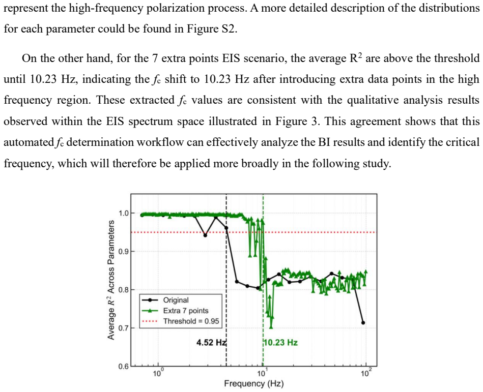
The central claim, stated in the paper's own terms, is that 'additional high-frequency sampling can not only shift fc to higher values but also reduce the total measurement time.' Concretely, when extra samples are inserted between neighboring high-frequency points (1, 3, 7, or 15 per interval) and those augmented spectra are fit with Bayesian inference over equivalent-circuit parameters, the inferred model can reproduce the low-frequency impedance semicircle that the partial spectrum no longer contains. In the proof-of-concept dual-RC example, adding 7 points lifts fc from 4.52 Hz to 10.23 Hz and visibly tightens the posterior predictive band at low frequency; across systematic tests, fc ri
Load-bearing premise
The extra high-frequency data are not experimental measurements but synthetic points generated from the very equivalent-circuit parameters the Bayesian fit is trying to estimate, so the claimed fc shift and time savings presuppose that the fitted model is exactly true and that the composite noise model captures reality.
Editorial extensions
If this is right
- For single-RC systems, the modeled time saving exceeds 98% at every tested noise level and densification, so this class of electrodes could in principle be screened with a short high-frequency-only sweep.
- For dual-RC systems (batteries, CO2 electrocatalysis), high-frequency densification still shifts fc upward and saves time in most conditions, but the benefit saturates and can reverse at 5% noise with 15 added points.
- The critical frequency is not a fixed property: it increases with added high-frequency points and decreases with noise, meaning the measurement window can be tuned per system using a once-per-system full-spectrum calibration.
- When the low-frequency semicircle dominates the polarization resistance (1:2 RC ratio), fc is highest, suggesting the skipped low-frequency process leaves a stronger trace in the high-frequency data.
- The workflow provides a quantitative stopping rule (three consecutive failed posterior checks) that can be automated, enabling adaptive truncation of the measurement.
Reading between the lines
- The entire demonstration is synthetic: extra points are generated from the optimized equivalent-circuit parameters and the same composite noise model used in fitting, so the reported fc shifts should be read as the behavior of a perfect-model world; a real measurement campaign with added experimental points is the necessary next test.
- A model-free version of this idea—using distribution-of-relaxation-times analysis or a nonparametric impedance model instead of a fixed ECM—would test whether high-frequency densification helps without assuming the circuit topology in advance.
- The uniform recursive subdivision is likely not information-optimal; placing extra points at frequencies where the Fisher information about the low-frequency parameters is largest could push fc further with the same number of added measurements.
- If the reconstruction holds on real cells, the method applies naturally to long-duration cycling studies where repeated full EIS scans are prohibitive, turning each cycle's check into a short high-frequency measurement plus an inference step.
Editorial analysis
A structured set of objections, weighed in public.
Referee Report
Summary. The paper proposes a Bayesian-inference framework for reducing the amount of low-frequency EIS data needed to recover a full impedance spectrum. The method adds synthetic high-frequency sampling points, fits the augmented partial spectrum with equivalent circuit models (ECMs) via AutoEIS, and introduces a critical frequency fc defined as the highest cutoff frequency at which the full response can still be reliably reconstructed. Reconstruction quality is judged by averaging Q-Q plot R² values of posterior parameter distributions. The authors report that high-frequency densification shifts fc to higher frequencies and reduces modeled measurement time, with single-RC systems saving over 98% of the time. All experiments are performed on synthetic data generated from the same ECMs used in fitting.
Significance. If the central claim were established, the work would be a practical contribution to accelerated EIS, with a useful organizing metric (fc) and a systematic study of noise level, densification, and ECM structure. The Bayesian fitting workflow is standard, the synthetic study covers multiple noise levels and random seeds, and the paper is clear about its use of synthetic data. However, the evidence is entirely self-referential: the extra high-frequency points are generated from the same optimized parameters that the Bayesian fit estimates, and the ground-truth spectra are generated from the same ECM used for fitting. The reported fc shifts and time savings are therefore currently statements about internal consistency in a synthetic world, not about transfer to real electrochemical measurements. With independent validation, the framework could be significant, but that validation is missing.
major comments (4)
- [Sec. 2.4 and Sec. 3.1] The additional high-frequency points are generated 'based on optimized ECM parameters and noise' (Sec. 2.4). This closes the loop: the densified data are drawn from the same parameter values that the Bayesian fit will estimate from the partial spectrum. The extra points therefore cannot carry any information beyond the model's own predictions plus the calibrated noise in Eq. (1). The observed fc shifts (e.g., 4.52 Hz to 10.53 Hz in Sec. 3.1) and the >98% single-RC time savings in Sec. 3.4 are thus self-consistency results. To make the central claim load-bearing, the extra points should come from independent ground-truth parameters fixed before fitting, or from real measurements; the limitation discussion in Sec. 5 mentions only uniform subdivision and does not acknowledge this closed-loop issue.
- [Sec. 2.2 and Sec. 3.1] The ground truth is generated from the same ECM (R1-[P2,R3] or R1-[P2,R3]-[P4,R5]) that is later fit to the data. This excludes model mismatch, unmodeled physical processes (e.g., diffusion, inductive artifacts), non-stationarity beyond the fitted drift, and instrument-specific noise statistics. The definition of fc as the frequency above which 'the full EIS response can still be reliably recovered' is therefore only meaningful within the assumed model. The paper should include at least one test where the data-generating ECM differs from the fitting ECM, or better, an experimental validation, to show that the reconstruction claim is not an artifact of model self-consistency.
- [Sec. 3.4, Eq. (2)] The time-saving formula in Eq. (2) is ambiguous. The text states the optimized measurement runs 'from the highest frequency to the critical frequency, fc,' but the equation sums ∑_{j=c}^{M} 1/f_j. If c is the index of fc in a descending-frequency array, the sum should run from the highest index to c (or j=1 to c with appropriate reindexing). As written, it is unclear whether the added high-frequency points are included in the numerator. The reported >98% single-RC time savings depend directly on this summation. Please clarify the indexing and re-derive the percentages.
- [Sec. 3.2 and Fig. 4] The fc criterion (average Q-Q R² > 0.95, with a three-consecutive-failure rule) is an indirect proxy for reconstruction quality. The paper validates it against only a single example (Fig. 4), comparing the R²-based fc to a qualitative visual assessment of the Nyquist predictions. To make fc a reliable metric, the authors should demonstrate, across multiple noise levels and densification factors, that the R² threshold corresponds to a direct error measure in the reconstructed low-frequency impedance (e.g., relative error in the omitted frequency range). Without this calibration, the reported fc values remain tied to an ad hoc threshold.
minor comments (6)
- [Sec. 3.4] The paragraph describing the time-calculation method is duplicated verbatim immediately before Eq. (2). One copy should be removed.
- [Sec. 3.4, text] Typo: 'reversely protentional' should be 'inversely proportional.' Also, the phrase 'data points and times' in Sec. 3.4 is unclear; consider 'the number of added data points and the resulting measurement time.'
- [Data and Code Availability] The statement that data and code 'will be made publicly available upon acceptance' is not sufficient for peer review. Please provide the code/scripts used for the synthetic generation, BI fitting, and fc determination as supplementary material, or at least include a detailed pseudo-code appendix.
- [Figures 5 and 6] The captions should explicitly state that error bands/error bars are mean±standard deviation over the four random seeds, and that the same random seeds were used for both synthetic data generation and inference. This is mentioned in the text but not in the captions.
- [Eq. (1)] Define the units and meaning of f in the flicker-noise term. Also clarify whether a, b, and c are fixed constants or tunable hyperparameters; the text says they are adjustable but only one set is used.
- [References] Several references are incomplete or non-standard (e.g., ref. 1 lacks author and journal details; ref. 36 appears to be an unpublished note). Please ensure all references follow the journal style and include complete bibliographic information.
Circularity Check
fc shift is a self-consistency result: added high-frequency points are generated from the same optimized ECM parameters the fit estimates, so the low-frequency 'reconstruction' is the model's own forward response.
-
self definitional
[Sections 2.2 and 2.4; claim in Abstract and Sec 3.1]
"we use noisy synthetic EIS data instead of noisy experimental data to efficiently obtain ground truth and systematically control the noise level ... We addressed shifts in the critical frequency, fc, by generating additional high-frequency data points based on optimized ECM parameters and noise."
The extra high-frequency points are generated from the same optimized ECM parameters that the Bayesian fit estimates, and the ground-truth full spectrum is generated from the same ECM (Sec 2.2). Thus the 'reconstruction' of low-frequency behavior is the forward model evaluated at the inferred parameters: it cannot fail due to model mismatch or unmodeled physics. The fc shift is therefore a measure of internal identifiability in a synthetic world, not an empirical prediction about real EIS. The closed loop is reinforced by Sec 3.3, which uses the same random seed for data generation and inference. The headline time saving is a direct consequence of this self-consistent fc shift.
full rationale
The paper's own equations close the loop. Section 2.2 states 'we use noisy synthetic EIS data instead of noisy experimental data to efficiently obtain ground truth and systematically control the noise level,' and Section 2.4 says the extra high-frequency points are 'generated ... based on optimized ECM parameters and noise.' Because those optimized parameters are exactly the target of the AutoEIS/Bayesian fit, and because the ground-truth full spectrum is generated from the same ECM, the 'reconstruction' of low-frequency behavior is the forward model evaluated at the inferred parameters. The reported fc shifts (e.g., dual-RC ~4.5 Hz to ~10.5 Hz in Sec 3.1) therefore measure parameter identifiability within the synthetic model class, not the ability to recover real unmeasured physics that is absent from the generator. This is a genuine circularity for the central empirical claim: densifying high-frequency data with model-generated points cannot reveal model mismatch, unmodeled diffusion/inductive/contact effects, or noise statistics beyond Eq. (1). The paper is transparent about the synthetic setup and does not claim experimental validation, but the conclusion that the framework 'challenges standard sampling paradigms' rests on this closed loop. The acknowledged limitation (Sec 5) concerns uniform subdivision, not the closed-loop generator. The self-citations to refs 10 and 26 for fc, the noise model, and AutoEIS are methodology inheritance, not a separate load-bearing circularity. Because the Bayesian inference itself is a real computation and densification genuinely improves identifiability in some cases, the circularity is partial: score 6.
Assumptions & free parameters
free parameters (5)
- Noise mixing ratios a, b, c =
a=0.01, b=0.01, c=10
- Global noise ratio eta =
0.01–0.05 (swept)
- Average Q-Q R2 threshold =
0.95
- Consecutive-failure count =
3
- Densification factors =
1, 3, 7, 15
assumptions (5)
- domain assumption The chosen equivalent circuit model (single-RC or dual-RC) is the correct data-generating process for the system.
- domain assumption The composite noise model (parameter drift + |Z|-proportional Gaussian + 1/f flicker) captures real EIS noise.
- ad hoc to paper Average Q-Q plot R2 across circuit parameters measures whether a partial spectrum carries enough information to reconstruct the full response.
- domain assumption Measurement time per frequency point is proportional to 1/f.
- ad hoc to paper Synthetic extra points derived from the fitted parameters behave like real additional high-frequency measurements.
invented entities (2)
-
Critical frequency fc
-
Noisy frequency threshold fn
Cite this review
Pith. "Pith review of Accelerating Electrochemical Impedance Spectroscopy Measurements by Reducing Reliance on Noisy Low-Frequency Data." pith.science (2026). https://pith.science/paper/PAAA35HG
@misc{pith2026260719307,
  author       = {Pith},
  title        = {Pith review of: Accelerating Electrochemical Impedance Spectroscopy Measurements by Reducing Reliance on Noisy Low-Frequency Data},
  year         = {2026},
  howpublished = {\url{https://pith.science/paper/PAAA35HG}},
  note         = {Machine review of arXiv:2607.19307}
}
read the original abstract
Electrochemical impedance spectroscopy (EIS) is a powerful tool for probing kinetic and transport processes in electrochemical systems, but its practical use is often limited by the long acquisition time and noise sensitivity of low-frequency measurements. Here, we present a statistical inference-assisted framework that reduces the reliance on low-frequency sampling by increasing the sampling density in cleaner high-frequency regions. Using AutoEIS and Bayesian inference, the augmented high-frequency data are fitted to selected equivalent circuit models (ECMs) to reconstruct the full impedance spectrum and quantify parameter uncertainty. To evaluate reconstruction performance, we introduce the critical frequency (fc), defined as the highest cutoff frequency at which the full EIS response can still be reliably recovered. The results show that additional high-frequency sampling can not only shift fc to higher values but also reduce the total measurement time. The specific improvement depends on the noise level of the EIS data, the number of added data points, and the ECM structure. Overall, this work provides a practical framework for designing fast and efficient EIS data acquisition and offers guidance for applying partial-frequency EIS reconstruction in real electrochemical characterization.
Figures


Figures from the paper (1 more)

Reference graph
Works this paper leans on
-
[6]
(38) Introduction to Statistical Quality Control, 8th Edition | Wiley
https://doi.org/10.1186/s40488-018-0088-5. (38) Introduction to Statistical Quality Control, 8th Edition | Wiley. Wiley.com. https://www.wiley.com/en- ca/Introduction+to+Statistical+Quality+Control%2C+8th+Edition-p-9781119399308 (accessed 2026-05-25). (39) Jaberi, A.; Sadeghi, M. A.; Zhang, R.; Zhao, Z.; Shi, Q.; Black, R.; Sadighi, Z.; Hattrick- Simpers,...
arXiv 2026
-
[101]
(6) Agarwal, P.; Orazem, M. E.; Garcia‐Rubio, L. H. Measurement Models for Electrochemical Impedance Spectroscopy: I . Demonstration of Applicability. J. Electrochem. Soc. 1992, 139 (7), 1917–1927. https://doi.org/10.1149/1.2069522. (7) Lazanas, A. Ch.; Prodromidis, M. I. Electrochemical Impedance Spectroscopy─A Tutorial. ACS Meas. Sci. Au 2023, 3 (3), 16...
arXiv 1992
-
[120]
(11) Ye, C.; Wang, M.-Q.; Bao, S.-J.; Ye, C
https://doi.org/10.1038/s41529-024-00537-8. (11) Ye, C.; Wang, M.-Q.; Bao, S.-J.; Ye, C. Micropore-Boosted Layered Double Hydroxide Catalysts: EIS Analysis in Structure and Activity for Effective Oxygen Evolution Reactions. ACS Appl. Mater. Interfaces 2019, 11 (34), 30887–30893. https://doi.org/10.1021/acsami.9b09144. (12) Choi, J.; Sim, J.; Oh, H.; Min, ...
-
[285]
https://doi.org/10.5006/1.3290350. (14) Berdimurodov, E.; Eliboyev, I.; Berdimuradov, K.; Kholikov, A.; Akbarov, K.; Dagdag, O.; Rbaa, M.; El Ibrahimi, B.; Verma, D. K.; Haldhar, R.; Arrousse, N. Chapter 3 - Electrochemical Impedance (EIS) and Noise Analyses for Corrosion Measurements. In Electrochemical and Analytical Techniques for Sustainable Corrosion...
-
[1491]
https://doi.org/10.3390/en14051491. (13) Cottis, R. A. Interpretation of Electrochemical Noise Data. Corrosion 2001, 57 (3), 265–
-
[1885]
(22) Abaspour, M.; Pattipati, K
https://doi.org/10.1149/1.2044210. (22) Abaspour, M.; Pattipati, K. R.; Shahrrava, B.; Balasingam, B. Robust Approach to Battery Equivalent-Circuit-Model Parameter Extraction Using Electrochemical Impedance Spectroscopy. Energies 2022, 15 (23),
-
[1993]
Pine Research Instrumentation Store
(3) Electrochemcal Impedance Spectroscopy (EIS) Basics. Pine Research Instrumentation Store. https://pineresearch.com/shop/kb/theory/eis-theory/eis-basics/ (accessed 2023-08-08). (4) Mansfeld, F.; Xiao, H.; Wang, Y. Evaluation of Localized Corrosion Phenomena with Electrochemical Impedance Spectroscopy (EIS) and Electrochemical Noise Analysis (ANA). Mater...
-
[2022]
https://doi.org/10.1007/978-981-19-4755-1. (36) Murphy, K. P. Conjugate Bayesian Analysis of the Gaussian Distribution. (37) Dytso, A.; Bustin, R.; Poor, H. V.; Shamai, S. Analytical Properties of Generalized Gaussian Distributions. J. Stat. Distrib. Appl. 2018, 5 (1),
Show all 9 references
-
[9251]
(23) Ulgut, B
https://doi.org/10.3390/en15239251. (23) Ulgut, B. Methods-Employing Multisine Electrochemical Impedance Spectroscopy for Batteries In Galvanostatic Mode. J. Electrochem. Soc. 2022, 169 (11), 110510. https://doi.org/10.1149/1945-7111/ac9d05. (24) Nam, K.-M.; Shin, D.-H.; Jung,...
2022
Reviewed August 1, 2026 · model on record in the stance chip above.
Discussion (0). Continue with ORCID to comment.