REVIEW 4 major objections 6 minor 107 references
High-redshift binary black holes can be inverted into a candidate bump in the small-scale primordial power spectrum.
Reviewed by Pith at T0; open to challenge. T0 means a machine referee read the full paper against a public rubric. the ladder, T0–T4 →
T0 review · grok-4.5
2026-07-14 06:44 UTC pith:PDUFBN4U
load-bearing objection Solid end-to-end inverse pipeline from redshifted BBH masses to small-scale PPS; the LVK bump is only a labeled illustration and should not be over-read. the 4 major comments →
Reconstruction of Primordial Power Spectrum from Gravitational Waves of High-Redshift Black Hole Binaries
The pith
A machine-rendered reading of the paper's core claim, the machinery that carries it, and where it could break.
Core claim
A gradient-descent inversion of the observed redshifted mass distribution of high-redshift binary black holes, followed by Tikhonov-regularized Press–Schechter inversion, yields a regularization-stable candidate bump-like enhancement of order O(10^{-2}) in the primordial power spectrum centered at k_peak ≃ 5.7 imes 10^5 Mpc^{-1} under the adopted assumptions, demonstrating that the reconstruction chain is feasible for next-generation detectors.
What carries the argument
The integral map (Eq. 19/20) that expresses the observed redshifted mass distribution P_O(m_1^z, m_2^z) as a double convolution of the PBH mass function f(m) with the binary-formation weight η, detector window W, and redshift distribution p(z); this map is inverted by gradient descent on a discretized mass vector, after which the Press–Schechter relation plus Tikhonov regularization recovers P_R(k).
Load-bearing premise
That the black-hole events kept after simple mass cuts can be treated as a pure primordial sample whose binaries form under the paper’s three simplifying assumptions and whose detection is captured by a circular-orbit signal-to-noise window.
What would settle it
A large, clean sample of binary black holes at z ≳ 20 whose reconstructed mass function shows no peak near tens of solar masses (or whose regularized power spectrum shows no corresponding O(10^{-2}) bump near 5 imes 10^5 Mpc^{-1}) would falsify the candidate feature under the same pipeline.
If this is right
- Next-generation detectors that accumulate high-redshift binaries can map the small-scale primordial power spectrum without relying on cosmic-microwave-background or large-scale-structure data.
- The same pipeline supplies an independent estimate of the total PBH dark-matter fraction once the merger abundance is matched.
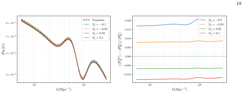
- Weak non-Gaussian corrections can be folded into the Press–Schechter step, shifting the reconstructed amplitude in a controlled, testable way.
- Consistency between independent mass cuts (e.g., m > 15 M_⊙ versus m > 50 M_⊙) becomes a built-in internal check on the reconstructed mass function.
Where Pith is reading between the lines
- Once Einstein Telescope or DECIGO catalogs exist, the identical inversion can be run in redshift slices to test whether the candidate bump is redshift-independent, as expected for a primordial feature.
- The method supplies a practical route to place joint constraints on both the amplitude and the width of any small-scale power-spectrum feature that produces solar-mass-scale PBHs.
- If late-time accretion or eccentricity systematically alter the observed mass distribution, the recovered peak position will drift; monitoring that drift with improved templates would diagnose the size of the neglected effects.
Editorial analysis
A structured set of objections, weighed in public.
Referee Report
Summary. The manuscript develops an inverse pipeline that reconstructs the PBH mass function f(m) from the observed redshifted-mass distribution of high-redshift BBHs via gradient descent on Eq. (20), then maps the resulting abundance through the Press–Schechter relation and a Tikhonov-regularized inverse convolution to the small-scale primordial power spectrum P_R(k). The forward map from f(m) to P(m_1^z, m_2^z) is derived under three early-universe assumptions (Poisson spatial distribution, common decoupling time, negligible late-time mass evolution), with a circular-orbit SNR>8 detector window. Uniqueness of the discretized mass-function inverse is argued in Appendix A. As an illustration, mass-selected LVK events (m>15 M_⊙, 174 events; m>50 M_⊙, 6 events) are treated as PBH candidates, yielding a lognormal-like f(m) peaking near ~20–35 M_⊙, f_PBH≃1.08×10^{-3}, and a regularization-stable candidate O(10^{-2}) bump in P_R(k) near k_peak≃5.7×10^5 Mpc^{-1}. Weak non-Gaussian (skewness) corrections are also explored. The stated goal is to demonstrate feasibility for next-generation detectors at z≳20.
Significance. If the pipeline is robust, it offers a concrete, data-driven route from high-redshift GW catalogs to the small-scale curvature spectrum—scales inaccessible to CMB/LSS—using next-generation detectors (ET, DECIGO, LISA, TianQin/Taiji). Strengths include a carefully derived forward relation (Eq. 19), an explicit uniqueness argument for the discretized inverse under positivity (Appendix A), transparent Tikhonov regularization with L-curve guidance (Appendix B), and public data availability. The high-z feasibility argument is the scientifically durable contribution; the LVK numbers are secondary and correctly flagged by the authors as illustrative rather than a definitive PBH detection.
major comments (4)
- Abstract and §VII present a “regularization-stable candidate bump-like enhancement of order O(10^{-2}) … centered around k_peak≃5.7×10^5 Mpc^{-1}” as a concrete finding, while §I and §V state that LVK events are not known to be PBHs and that the exercise is only for illustration. The numerical feature is load-bearing for how the paper will be cited. Please either (i) demote the LVK bump to a clearly labeled mock/illustrative result in the abstract and conclusions, or (ii) add a quantitative contamination test: inject a controlled astrophysical fraction into the m>15 M_⊙ sample and show how the reconstructed f(m) peak and P_R bump degrade. Without this, the abstract overstates what the LVK application can support.
- §III assumptions 1–3 (Poisson spatial distribution, common t_dec, negligible late-time mass evolution) and the circular-orbit window of Eqs. (24)–(35) are used both for the method and for the LVK illustration. The text correctly defers accretion, disruption, three-body capture, and eccentricity to future work, but these effects enter the kernel that is inverted. For the feasibility claim aimed at next-generation detectors, a short robustness subsection (or appendix) is needed: e.g., how a 10–30% late-time mass shift or a non-Poisson clustering term biases the recovered f(m) and the subsequent P_R peak. Without it, the mapping from high-z catalogs to P_R remains unquantified under realistic deviations from the three assumptions.
- §VI, after Eq. (50): the reconstruction identifies the collapse fraction β(M) with the abundance in each mass bin, “valid for sharply peaked spectra,” with a more accurate differential/excursion-set treatment left for future work. The reconstructed f(m) is lognormal-like with σ_MF~0.5–0.8 (Table I), not infinitely sharp. This approximation directly sources σ^2(R) and therefore the location and amplitude of the reported P_R bump. Please quantify the bias (e.g., by comparing the bin-identification prescription to dβ/dlnM or a simple excursion-set estimate on the same f(m)), or restrict the PPS claim to the sharply-peaked limit and state the systematic floor on k_peak and β_p.
- §V, Eq. (42): f_PBH is fixed by requiring N_PBH(f_PBH)=174 for the m>15 M_⊙ sample. The shape of f(m) comes from the redshifted-mass inversion, but the overall amplitude that enters β(m) and thus P_R is set by this match. Please report the sensitivity of the reconstructed P_R amplitude to a factor-of-few variation in the adopted merger-rate formula (Eq. 40) and to the choice of which events are counted as PBH candidates, so that the O(10^{-2}) height is not read as uniquely determined by the data.
minor comments (6)
- Fig. 3 and Table I: the power-law fit α_MF=1.56 is quoted for the combined sample, but the right panel of Fig. 3 shows it only over a limited range; clarify the mass interval used for each fit and whether the reduced χ^2_ν accounts for the full covariance of the 100 reconstruction draws.
- Eq. (19) vs. Eq. (20): the switch from P to P_O / f_p is clear in the text but the notation for the physical vs. assumed mass function (f_p vs. f̃) is easy to lose in later sections; a short notation table or consistent subscripts would help.
- §V: pastro≥0.9 is used as a selection cut; pastro does not distinguish stellar vs. primordial origin. A one-sentence reminder of this limitation next to the cut definition would avoid misreading.
- Fig. 4: the IR non-decaying tail is correctly caveated in the text; adding a vertical band marking the k-range that is actually constrained by the reconstructed mass interval would make the figure self-contained.
- Appendix A: the uniqueness argument is for the equal-mass slice m_1^z=m_2^z and for a fixed regularization operator L and λ. A brief remark that the full two-dimensional (m_1^z,m_2^z) inverse inherits uniqueness under the same positivity and fixed-(L,λ) conditions would close the loop with the gradient-descent procedure of §IV.
- References: GWTC-4/5 arXiv numbers and the 2025–2026 LVK papers are cited; ensure final published versions are updated at proof stage if available.
Circularity Check
No significant circularity: the pipeline is a regularized inverse problem (redshifted masses to f(m) via gradient descent, then Press-Schechter + Tikhonov to PR(k)); the LVK abundance scale is calibrated to the selected sample size, which is ordinary reconstruction under stated assumptions rather than a tautology.
full rationale
The claimed chain (mz1,mz2)obs → PO → f(m) → fPBH(m) → β → σ² → PR(k) is an explicit inverse problem. Gradient descent minimizes the discrepancy between the model PO of Eq. (20)/(21) and the observed redshifted-mass histogram; uniqueness of the discretized map is proved self-containedly in Appendix A (positive kernel + positivity of f). The subsequent Press-Schechter steps are arithmetic plus a standard Tikhonov regularized inverse convolution (Eqs. 58–62), with λ chosen by the L-curve (Appendix B). The only data-driven scale is the overall fPBH fixed by requiring NPBH(fPBH)=174 (Eq. 42) for the m>15 M⊙ cut; that normalizes the amplitude of β and therefore of PR, but does not force the location or existence of the mass-function peak (which is read from the data) nor the subsequent bump at kpeak≃5.7×10^5 Mpc^{-1}. The paper repeatedly labels the LVK exercise “illustrative”/“benchmark” under the three Sec. III assumptions and the circular-orbit window, so the numerical feature is not presented as a model-independent prediction. Self-citations to earlier reconstruction papers by overlapping authors supply context but are not load-bearing for uniqueness or for the inversion itself. Hence the derivation does not reduce to its inputs by construction.
Axiom & Free-Parameter Ledger
free parameters (6)
- mass-selection thresholds (15 M_⊙ and 50 M_⊙) =
15 M_⊙ / 50 M_⊙
- f_PBH (overall abundance) =
1.08 × 10^{-3}
- Tikhonov regularization strength λ =
10^{-5} to 10^{-1}
- collapse threshold δ_c =
0.45
- collapse efficiency γ_m and g_* =
γ_m=0.2, g_*=10.75
- learning rate γ of gradient descent
axioms (5)
- domain assumption Initial PBH spatial distribution is Poisson; binaries decouple at a common early time t_dec; late-time mass evolution is negligible.
- domain assumption Press-Schechter formalism with Gaussian (or weakly non-Gaussian) density contrast and a fixed threshold δ_c maps σ^{2}(R) to the collapse fraction β(m).
- domain assumption Detector window function can be approximated by circular-orbit SNR>8 and a critical-frequency cut derived from 10-year LVK evolution (Eqs. 24–35).
- standard math Discretized inverse problem for the mass function is unique under positivity of f(m) (Appendix A).
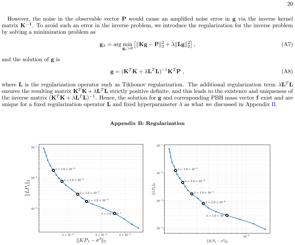
- ad hoc to paper Tikhonov regularization with first- or second-order difference operators yields a stable, physically acceptable P_R(k).
invented entities (2)
-
discrete PBH mass-distribution vector f and its gradient-descent update rule
no independent evidence
-
reconstruction matrix R_λ = (K^T K + λ L^T L)^{-1} K^T
no independent evidence
read the original abstract
High-redshift binary black hole (BBH) events are promising candidates for primordial black holes (PBHs) detectable by next-generation gravitational wave (GW) detectors. A redshifted mass distribution of detected PBH candidates can be obtained from GW observations, from which the underlying PBH mass function can be reconstructed. In this work, we develop a framework that applies the gradient-descent method to the observed redshifted mass distribution and reconstructs the PBH mass function and, subsequently, the primordial power spectrum (PPS) on small scales. As an illustrative application, we analyze BBH events in the LIGO--Virgo--KAGRA (LVK) catalogs under a specified PBH selection criterion. We find a regularization-stable candidate bump-like enhancement of order $\mathcal{O}(10^{-2})$ in the reconstructed PPS, centered around $k_{\mathrm{peak}}\simeq 5.7\times 10^5~\mathrm{Mpc}^{-1}$ under the adopted assumptions. Our results demonstrate the feasibility of reconstructing the small-scale PPS from high-redshift BBH observations with next-generation GW detectors.
Figures


Reference graph
Works this paper leans on
-
[1]
The reconstructed mass function, together with the observed merger abundance determines the total PBH fraction fPBH
→ f(m) using gradient-descent method. The reconstructed mass function, together with the observed merger abundance determines the total PBH fraction fPBH. Finally, using Press-Schechter relation, fPBH(m) is converted into the collapse fraction β(m), then into the variance of the smoothed density contrast σ2(R), and ultimately into the primordial curvature...
-
[2]
⇒ f(m) ⇒ fPBH(m) ⇒ β(m) ⇒ σ2(R) ⇒ P R(k). (1) III. REDSHIFTED MASS DISTRIBUTION OF OBSERVED PBH BINARIES AT HIGH REDSHIFTS In the following discussion, we focus on developing a formalism that connects the observed redshifted mass distri- bution of PBH binaries with the PBH mass function, and use this formalism to extract PBH mass function from the GW obse...
-
[3]
The initial PBH spatial distribution follows the Poisson distribution
-
[4]
PBH binaries decouple from the background Hubble flow at the same cosmic time tdec which is early enough
-
[5]
From GW waveform of PBH binaries, we can extract the redshifted mass of PBHs mz, which is a combination of their redshift and intrinsic mass follows mz = (1 + z)m [41]
The initial PBH mass function has negligible late time evolution. From GW waveform of PBH binaries, we can extract the redshifted mass of PBHs mz, which is a combination of their redshift and intrinsic mass follows mz = (1 + z)m [41]. With the development of the next-generation GW detectors, such as Einstein Telescope [17], LISA [19], DECIGO [18], etc., t...
-
[6]
After detecting enough high-redshift BBH events, a redshifted mass distribution of PBH binaries P (mz 1, mz
can be obtained from two BH components 1. After detecting enough high-redshift BBH events, a redshifted mass distribution of PBH binaries P (mz 1, mz
-
[7]
can be statistically constructed, which is defined as follows, P (mz 1, mz
-
[8]
= 1 Ntot dNobs(mz 1, mz 2) dmz 1 dmz 2 , (2) where dNobs(mz 1, mz
-
[9]
is the number of observed PBH binaries within redshifted mass range ( mz 1, mz 1 + dmz
-
[10]
and (mz 2, mz 2 + dmz
-
[11]
Here, we should notice that the redshifted mass distribution of PBH binaries P (mz 1, mz
on the past light cone, Ntot is the total number of PBH binaries on the past light cone, mz 1 and mz 2 are the redshifted mass of each PBH component in binaries. Here, we should notice that the redshifted mass distribution of PBH binaries P (mz 1, mz
-
[12]
Intuitively, the observed redshifted mass distribution of PBH binaries depends on PBH mass function, sensitivity of GW detectors, and redshift distribution of PBH binaries
is not normalized, which means Ntot > RR dNobs dmz 1 dmz 2 dmz 1dmz 2 = Nobs. Intuitively, the observed redshifted mass distribution of PBH binaries depends on PBH mass function, sensitivity of GW detectors, and redshift distribution of PBH binaries. To find this relation, we start from calculating the cumulative distribution of redshifted PBH mass C(mz 1...
-
[13]
can be described as follows, C(mz 1, mz
-
[14]
= Nobs(ma < m z 1, mb < m z 2) Ntot = Z mz 1 0 Z mz 2 0 P (ma, mb)dmadmb , (3) where Nobs(ma < m z 1, mb < m z
-
[15]
To express C(mz 1, mz
is the number of observed PBH binaries with the redshifted mass of their components smaller than mz 1 and mz 2. To express C(mz 1, mz
-
[16]
Therefore PBH mass function is normalized asR f(m)dm = 1
in the form of PBH mass function f(m), we first define PBH mass function f(m) as the quantity f(m)dm is the probability that a randomly chosen PBH lies in the mass range ( m, m + dm), it can be expressed in the form of the PBH number density distribution as follows, f(m) = 1 nPBH dn dm , (4) where dn denotes the comoving number density of PBHs in the mass...
-
[17]
(13) To evaluate C(mz 1, mz 2), we first calculate its contribution within redshift range ( z, z + dz)
as dC(mz 1, mz 2) dm1dm2dz = 1 Ntot dN z obs(m1, m2) dm1dm2dz = f(m1)f(m2)η(m1, m2)p(z)W (m1, m2; z) . (13) To evaluate C(mz 1, mz 2), we first calculate its contribution within redshift range ( z, z + dz). For a given redshift z, the counted PBH binaries should satisfy that their intrinsic mass are in the range of (0 , mz 1/1 + z) and (0, mz 2/1 + z), th...
-
[18]
(15) Here we formally integrate redshift in the range of (0 , ∞) and (0 , mz/1 + z)
= Z ∞ 0 Z mz 1 1+z 0 Z mz 2 1+z 0 f(m1)f(m2)η(m1, m2)W (m1, m2; z)p(z)dm1dm2dz . (15) Here we formally integrate redshift in the range of (0 , ∞) and (0 , mz/1 + z). However, in practice, the bound of integration should be in a physical range like ( mmin, mz/1 + z) which is determined by PBH mass distribution, and (zmin, zmax) which is determined by the G...
-
[19]
can be calculated by deriving the cumulative distribution with respect to the redshifted mass as P (mz 1, mz
-
[20]
(16) We first take the partial derivative of C(mz 1, mz
= ∂2C(mz 1, mz 2) ∂mz 1∂mz 2 . (16) We first take the partial derivative of C(mz 1, mz
-
[21]
with respect to mz 2 as follows, ∂C(mz 1, mz 2) ∂mz 2 = lim ∆mz 2 →0 1 ∆mz 2 Z ∞ 0 p(z)dz Z mz 1 1+z 0 f(m1)dm1 × Z mz 2+∆mz 2 1+z 0 f(m2)η(m1, m2)W (m1, m2; z)dm2 − Z mz 2 1+z 0 f(m2)η(m1, m2)W (m1, m2; z)dm2 = lim ∆mz 2 →0 1 ∆mz 2 Z ∞ 0 p(z)dz Z mz 1 1+z 0 f(m1)dm1 Z mz 2+∆mz 2 1+z mz 2 1+z f(m2)η(m1, m2)W (m1, m2; z)dm2 = Z ∞ 0 p(z)dz Z mz 1 1+...
-
[22]
as follows, P (mz 1, mz
-
[23]
= ∂2C(mz 1, mz 2) ∂mz 1 ∂mz 2 = Z ∞ 0 f mz 1 1 + z f mz 2 1 + z η mz 1 1 + z , mz 2 1 + z W mz 1 1 + z , mz 2 1 + z ; z p(z) (1 + z)2 dz . (19) Eq. (19) provides a direct relation between observed redshifted mass distribution and PBH mass function, this indicates that primordial physics from PBH mass function can be extracted from GW observations. However...
-
[24]
= Z ∞ 0 fp mz 1 1 + z fp mz 2 1 + z η mz 1 1 + z , mz 2 1 + z W mz 1 1 + z , mz 2 1 + z ; z p(z) (1 + z)2 dz , (20) where PO(mz 1, mz
-
[25]
Apart from fp(m), PO(mz 1, mz
with subscript O denotes the observed redshifted mass distribution and fp(m) is the physical PBH mass function. Apart from fp(m), PO(mz 1, mz
-
[26]
Once we know the contribution of W (m1, m2; z) and p(z), the physical PBH mass function fp(m) can be inversely solved from observed redshifted mass distribution PO(mz 1, mz 2)
only depends on detector-dependent window function W (m1, m2; z) and redshift distribution of PBH binaries p(z). Once we know the contribution of W (m1, m2; z) and p(z), the physical PBH mass function fp(m) can be inversely solved from observed redshifted mass distribution PO(mz 1, mz 2). It should be noticed that in constructing PO(mz 1, mz
-
[27]
from data, we first normalize PO(mz 1, mz
-
[28]
Solving PBH mass function in Eq
to facilitate numerical implementation, and this would introduce an artificial overall scaling factor on the physical PBH mass functionfp(m), then we recover the physical distribution of fp(m) by re-normalizing its reconstructed result. Solving PBH mass function in Eq. (20) is a typical inverse problem, which is hard to find an analytical solution. Hence,...
-
[29]
Give an initial PBH mass distribution as an initial condition of PBH mass function
-
[30]
Calculate theoretical redshifted mass distribution and compare it with observed one to obtain the error function
-
[31]
Update PBH mass function by calculating the gradient of error function with respect to the variation of PBH mass function. 7
-
[32]
Iterate PBH mass function until finding the minimum of error function, which is a best-fit approximation of physical PBH mass function. In order to reduce the computational cost of this algorithm, we start from discretizing PBH mass function f(m) to a PBH mass distribution vector f, where the component of vector follows fi = f(mi) and a set of {mi|1 ≤ i ≤...
-
[33]
= Z ∞ 0 ˜f mz 1 1 + z ˜f mz 2 1 + z η mz 1 1 + z , mz 2 1 + z W mz 1 1 + z , mz 2 1 + z ; z p(z) (1 + z)2 dz , (21) Then we can define an error function E(f) by comparing theoretical distribution with the observed redshifted mass distribution at a selected set of PBH binary mass pairs as follows [46], E(f) ≡ sP 1≤i≤j≤N[PT (mz i , mz j) − PO(mz i , mz j)]2...
-
[34]
are theoretical and observed redshifted mass distribution, respectively, and N is the number of selected redshifted mass points for mz 1 and mz 2. The error function E(f) only depends on the assumed PBH mass distribution vector f, so any further deviation of f from the physical PBH mass function fp(m) would enhance the difference between PT (mz 1, mz
-
[35]
and increase the value of error function. It indicates that, in order to minimize the difference between assumed PBH mass distribution vector and the physical PBH mass function, minimizing the error function E(f) could be an indicator to make f approach the physical PBH mass function. To minimize the error function E(f), we use the following iteration equ...
2015
-
[36]
plane is shown in Fig. 2. To model the probability distribution of the redshifted mass, we impose the split-normal distribution as an approximated distribution of masses involved each event, and the parameters of distribution are set as µ = mz i and σ± = σz i±/1.645, where we transfer 90% credible interval σz i± in the redshifted mass to the standard devi...
2000
-
[37]
It should be noticed that by modeling mz 1 and mz 2 as independent split-normal distribution, we have neglected their covariance
with corresponding 90% credible interval. It should be noticed that by modeling mz 1 and mz 2 as independent split-normal distribution, we have neglected their covariance. Since the current LVK measurement uncertainty is large, this split-normal distribution can be viewed as a conservative choice to model the probability distribution of the redshifted mas...
-
[38]
Then we reconstruct PBH mass function from redshifted mass distribution via gradient- descent method
for each PBH binary event, and this process produces various redshifted mass distribution for each round of PBH mass function reconstruction. Then we reconstruct PBH mass function from redshifted mass distribution via gradient- descent method. We repeat this process for 100 times so that 100 PBH mass functions will be produced. We set the number of round ...
-
[39]
(A1) In this proof, We understand it from the data reconstruction perspective by discretizing PBH mass function and kernel function and then Eq
= Z zmax zmin fp mz 1 1 + z fp mz 2 1 + z η mz 1 1 + z , mz 2 1 + z W mz 1 1 + z , mz 2 1 + z ; z p(z) (1 + z)2 dz . (A1) In this proof, We understand it from the data reconstruction perspective by discretizing PBH mass function and kernel function and then Eq. A1 can be transferred to a matrix equation. To simplify our consideration, we set mz 1 = mz 2 =...
-
[40]
(2) PO(mz 1, mz
Redshifted mass distribution of PBH binaries Eq. (2) PO(mz 1, mz
-
[41]
(1) C(mz 1, mz
Observed redshifted mass distribution of PBH binaries Eq. (1) C(mz 1, mz
-
[42]
(3) Nobs Observed number of PBH binaries on the past light cone Eq
Cumulative distribution of redshifted mass of PBH binaries Eq. (3) Nobs Observed number of PBH binaries on the past light cone Eq. (2) Ntot Total number of PBH binaries on the past light cone Eq. (2) Nz(m1, m2) The number of PBH binaries of ( m1,m2) on the past light cone Eq. (10) dn Comoving number density of PBHs in the mass range ( m, m + dm) Eq. (4) n...
-
[43]
Gravitationally collapsed objects of very low mass,
S. Hawking, “Gravitationally collapsed objects of very low mass,” Mon. Not. Roy. Astron. Soc. 152 (1971) 75
1971
-
[44]
The Hypothesis of Cores Retarded during Expansion and the Hot Cosmological Model,
Y. B. Zel’dovich and I. D. Novikov, “The Hypothesis of Cores Retarded during Expansion and the Hot Cosmological Model,” Sov. Astron. 10 (1967) 602
1967
-
[45]
Black holes in the early Universe,
B. J. Carr and S. W. Hawking, “Black holes in the early Universe,” Mon. Not. Roy. Astron. Soc. 168 (1974) 399–415
1974
-
[46]
The behaviour of point masses in an expanding cosmological substratum,
P. Meszaros, “The behaviour of point masses in an expanding cosmological substratum,” Astron. Astrophys. 37 (1974) 225–228
1974
-
[47]
The Primordial black hole mass spectrum,
B. J. Carr, “The Primordial black hole mass spectrum,” Astrophys. J. 201 (1975) 1–19
1975
-
[48]
R. Kimura, T. Suyama, M. Yamaguchi, and Y.-L. Zhang, “Reconstruction of Primordial Power Spectrum of curvature perturbation from the merger rate of Primordial Black Hole Binaries,” JCAP 04 (2021) 031, arXiv:2102.05280 [astro-ph.CO]
Pith/arXiv arXiv 2021
-
[49]
X. Wang, Y.-l. Zhang, R. Kimura, and M. Yamaguchi, “Reconstruction of power spectrum of primordial curvature perturbations on small scales from primordial black hole binaries scenario of LIGO/VIRGO detection,” Sci. China Phys. Mech. Astron. 66 no. 6, (2023) 260462, arXiv:2209.12911 [astro-ph.CO]
Pith/arXiv arXiv 2023
-
[50]
Observation of Gravitational Waves from a Binary Black Hole Merger,
LIGO Scientific, Virgo Collaboration, B. P. Abbott et al., “Observation of Gravitational Waves from a Binary Black Hole Merger,” Phys. Rev. Lett. 116 no. 6, (2016) 061102, arXiv:1602.03837 [gr-qc]
Pith/arXiv arXiv 2016
-
[51]
GW190425: Observation of a Compact Binary Coalescence with Total Mass ∼ 3.4M⊙,
LIGO Scientific, Virgo Collaboration, B. P. Abbott et al., “GW190425: Observation of a Compact Binary Coalescence with Total Mass ∼ 3.4M⊙,” Astrophys. J. Lett. 892 no. 1, (2020) L3, arXiv:2001.01761 [astro-ph.HE]
Pith/arXiv arXiv 2020
-
[52]
LIGO Scientific, Virgo Collaboration, R. Abbott et al., “GW190814: Gravitational Waves from the Coalescence of a 23 Solar Mass Black Hole with a 2.6 Solar Mass Compact Object,” Astrophys. J. Lett. 896 no. 2, (2020) L44, 23 arXiv:2006.12611 [astro-ph.HE]
Pith/arXiv arXiv 2020
-
[53]
S. Clesse and J. Garcia-Bellido, “GW190425, GW190521 and GW190814: Three candidate mergers of primordial black holes from the QCD epoch,” Phys. Dark Univ. 38 (2022) 101111, arXiv:2007.06481 [astro-ph.CO]
Pith/arXiv arXiv 2022
-
[54]
GW190521: A Binary Black Hole Merger with a Total Mass of 150M⊙,
LIGO Scientific, Virgo Collaboration, R. Abbott et al., “GW190521: A Binary Black Hole Merger with a Total Mass of 150M⊙,” Phys. Rev. Lett. 125 no. 10, (2020) 101102, arXiv:2009.01075 [gr-qc]
arXiv 2020
-
[55]
GW231123: A Binary Black Hole Merger with Total Mass 190–265 M⊙,
LIGO Scientific, VIRGO, KAGRA Collaboration, A. G. Abac et al., “GW231123: A Binary Black Hole Merger with Total Mass 190–265 M⊙,” Astrophys. J. Lett. 993 no. 1, (2025) L25, arXiv:2507.08219 [astro-ph.HE]
Pith/arXiv arXiv 2025
-
[56]
GW190521 Mass Gap Event and the Primordial Black Hole Scenario,
V. De Luca, V. Desjacques, G. Franciolini, P. Pani, and A. Riotto, “GW190521 Mass Gap Event and the Primordial Black Hole Scenario,” Phys. Rev. Lett. 126 no. 5, (2021) 051101, arXiv:2009.01728 [astro-ph.CO]
Pith/arXiv arXiv 2021
-
[57]
GW231123 mass gap event and the primordial black hole scenario,
C. Yuan, Z.-C. Chen, and L. Liu, “GW231123 mass gap event and the primordial black hole scenario,” Phys. Rev. D 112 no. 8, (2025) L081306, arXiv:2507.15701 [astro-ph.CO]
arXiv 2025
-
[58]
Detectability of primordial black hole binaries at high redshift,
Q. Ding, “Detectability of primordial black hole binaries at high redshift,” Phys. Rev. D 104 no. 4, (2021) 043527, arXiv:2011.13643 [astro-ph.CO]
Pith/arXiv arXiv 2021
-
[59]
The Einstein Telescope: A third-generation gravitational wave observatory,
M. Punturo et al., “The Einstein Telescope: A third-generation gravitational wave observatory,” Class. Quant. Grav. 27 (2010) 194002
2010
-
[60]
The Japanese space gravitational wave antenna: DECIGO,
S. Kawamura et al., “The Japanese space gravitational wave antenna: DECIGO,” Class. Quant. Grav. 28 (2011) 094011
2011
-
[61]
Laser Interferometer Space Antenna,
LISA Collaboration, P. Amaro-Seoane et al., “Laser Interferometer Space Antenna,” arXiv:1702.00786 [astro-ph.IM]
-
[62]
TianQin: a space-borne gravitational wave detector,
TianQin Collaboration, J. Luo et al., “TianQin: a space-borne gravitational wave detector,” Class. Quant. Grav. 33 no. 3, (2016) 035010, arXiv:1512.02076 [astro-ph.IM]
Pith/arXiv arXiv 2016
-
[63]
The Taiji Program in Space for gravitational wave physics and the nature of gravity,
W.-R. Hu and Y.-L. Wu, “The Taiji Program in Space for gravitational wave physics and the nature of gravity,” Natl. Sci. Rev. 4 no. 5, (2017) 685–686
2017
-
[64]
Science with the space-based interferometer eLISA: Supermassive black hole binaries,
A. Klein et al., “Science with the space-based interferometer eLISA: Supermassive black hole binaries,” Phys. Rev. D 93 no. 2, (2016) 024003, arXiv:1511.05581 [gr-qc]
Pith/arXiv arXiv 2016
-
[65]
T. Nakamura et al., “Pre-DECIGO can get the smoking gun to decide the astrophysical or cosmological origin of GW150914-like binary black holes,” PTEP 2016 no. 9, (2016) 093E01, arXiv:1607.00897 [astro-ph.HE]
Pith/arXiv arXiv 2016
-
[66]
K. K. Y. Ng, G. Franciolini, E. Berti, P. Pani, A. Riotto, and S. Vitale, “Constraining High-redshift Stellar-mass Primordial Black Holes with Next-generation Ground-based Gravitational-wave Detectors,” Astrophys. J. Lett. 933 no. 2, (2022) L41, arXiv:2204.11864 [astro-ph.CO]
Pith/arXiv arXiv 2022
-
[67]
Science with the TianQin observatory: Preliminary results on massive black hole binaries,
H.-T. Wang et al., “Science with the TianQin observatory: Preliminary results on massive black hole binaries,” Phys. Rev. D 100 no. 4, (2019) 043003, arXiv:1902.04423 [astro-ph.HE]
Pith/arXiv arXiv 2019
-
[68]
Taiji program: Gravitational-wave sources,
W.-H. Ruan, Z.-K. Guo, R.-G. Cai, and Y.-Z. Zhang, “Taiji program: Gravitational-wave sources,” Int. J. Mod. Phys. A 35 no. 17, (2020) 2050075, arXiv:1807.09495 [gr-qc]
Pith/arXiv arXiv 2020
-
[69]
Properties of the Binary Black Hole Merger GW150914,
LIGO Scientific, Virgo Collaboration, B. P. Abbott et al., “Properties of the Binary Black Hole Merger GW150914,” Phys. Rev. Lett. 116 no. 24, (2016) 241102, arXiv:1602.03840 [gr-qc]
Pith/arXiv arXiv 2016
-
[70]
An overview of gradient descent optimization algorithms,
S. Ruder, “An overview of gradient descent optimization algorithms,” arXiv e-prints (Sept., 2016) arXiv:1609.04747, arXiv:1609.04747 [cs.LG]
Pith/arXiv arXiv 2016
-
[71]
Merger rate of primordial black hole binaries as a probe of the Hubble parameter,
Q. Ding, “Merger rate of primordial black hole binaries as a probe of the Hubble parameter,” Phys. Rev. D 110 no. 6, (2024) 063542, arXiv:2312.13728 [astro-ph.CO]
Pith/arXiv arXiv 2024
-
[72]
LIGO Scientific, Virgo Collaboration, B. P. Abbott et al., “GWTC-1: A Gravitational-Wave Transient Catalog of Compact Binary Mergers Observed by LIGO and Virgo during the First and Second Observing Runs,” Phys. Rev. X 9 no. 3, (2019) 031040, arXiv:1811.12907 [astro-ph.HE]
Pith/arXiv arXiv 2019
-
[73]
LIGO Scientific, Virgo Collaboration, R. Abbott et al., “GWTC-2: Compact Binary Coalescences Observed by LIGO and Virgo During the First Half of the Third Observing Run,” Phys. Rev. X 11 (2021) 021053, arXiv:2010.14527 [gr-qc]
Pith/arXiv arXiv 2021
-
[74]
KAGRA, VIRGO, LIGO Scientific Collaboration, R. Abbott et al., “GWTC-3: Compact Binary Coalescences Observed by LIGO and Virgo during the Second Part of the Third Observing Run,” Phys. Rev. X 13 no. 4, (2023) 041039, arXiv:2111.03606 [gr-qc]
Pith/arXiv arXiv 2023
-
[75]
LIGO Scientific, VIRGO, KAGRA Collaboration, A. G. Abac et al., “GWTC-4.0: Updating the Gravitational-Wave Transient Catalog with Observations from the First Part of the Fourth LIGO-Virgo-KAGRA Observing Run,” arXiv:2508.18082 [gr-qc]
-
[76]
GWTC-5.0: An Introduction to Version 5.0 of the Gravitational-Wave Transient Catalog,
LIGO Scientific, VIRGO, KAGRA Collaboration, A. G. Abac et al., “GWTC-5.0: An Introduction to Version 5.0 of the Gravitational-Wave Transient Catalog,” arXiv:2605.27223 [gr-qc]
-
[77]
A. Tanikawa, T. Yoshida, T. Kinugawa, A. A. Trani, T. Hosokawa, H. Susa, and K. Omukai, “Merger Rate Density of Binary Black Holes through Isolated Population I, II, III and Extremely Metal-poor Binary Star Evolution,” Astrophys. J. 926 no. 1, (2022) 83, arXiv:2110.10846 [astro-ph.HE]
Pith/arXiv arXiv 2022
-
[78]
Mind the Gap: The Location of the Lower Edge of the Pair-instability Supernova Black Hole Mass Gap,
R. Farmer, M. Renzo, S. E. de Mink, P. Marchant, and S. Justham, “Mind the Gap: The Location of the Lower Edge of the Pair-instability Supernova Black Hole Mass Gap,” Astrophys. J. 887 no. 1, (Dec., 2019) 53, arXiv:1910.12874 [astro-ph.SR]
Pith/arXiv arXiv 2019
-
[79]
R. Farmer, M. Renzo, S. de Mink, M. Fishbach, and S. Justham, “Constraints from gravitational wave detections of binary black hole mergers on the 12C (α, γ)16O rate,” Astrophys. J. Lett. 902 no. 2, (2020) L36, arXiv:2006.06678 [astro-ph.HE]
Pith/arXiv arXiv 2020
-
[80]
The Pair-Instability Mass Gap for Black Holes,
S. E. Woosley and A. Heger, “The Pair-Instability Mass Gap for Black Holes,” Astrophys. J. Lett. 912 no. 2, (2021) L31, arXiv:2103.07933 [astro-ph.SR] . 24
Pith/arXiv arXiv 2021
discussion (0)
Sign in with ORCID, Apple, or X to comment. Anyone can read and Pith papers without signing in.