Analytic Planetary Transit Light Curves and Derivatives for Stars with Polynomial Limb Darkening

Daniel Foreman-Mackey; Eric Agol; Rodrigo Luger

REVIEW 2 major objections 4 minor 1 cited by

Analytic Planetary Transit Light Curves and Derivatives for Stars with Polynomial Limb Darkening

T0 review · 2 major / 4 minor · reviewed 2026-08-14 · deepseek-v4-flash

Challenge this review Re-run · record.json Download PDF Read on arXiv ↗ Review JSON

Pith's one-line read For polynomial limb darkening of any integer order, the transit light curve is closed-form, stable, and differentiable.

desk verdict A carefully derived, well-validated analytic transit model with gradients for arbitrary integer-order polynomial limb darkening; the central result is solid and the minor exposition gaps do not undermine it. read the letter →

arxiv 1908.03222 v2 pith:PLPCBM3M submitted 2019-08-08 astro-ph.EP astro-ph.IM

Eric Agol , Rodrigo Luger , Daniel Foreman-Mackey This is my paper · ORCID

classification astro-ph.EPastro-ph.IM

keywords transitlightcurveslimbdarkeningoccultationclosed-formsolutionellipticintegralsnumericalstabilityanalyticderivativesexoplanetphotometry

verification ladder T0 review T1 audit T2 compute T3 formal

The pith

A machine-rendered reading of the paper's core claim, the machinery that carries it, and where it could break.

The reading

This paper claims that the transit or occultation light curve of a star with polynomial limb darkening is not limited to the usual linear and quadratic cases: for any integer order N, the flux is a closed-form expression built from a solution vector that depends only on the radius ratio and impact parameter. The same construction yields analytic partial derivatives of the flux with respect to the radius ratio, impact parameter, and all limb-darkening coefficients. A sympathetic reader would care because the formulas are designed to stay numerically stable precisely where earlier analytic models lose precision, near ingress and egress contacts and when the planet's edge crosses the star's center, and because the derivatives make gradient-based fitting and Hamiltonian Monte Carlo practical. The paper also shows that finite-exposure, time-averaged fluxes and their derivatives can be computed accurately, and that the model applies to eclipsing binaries and multiple-star systems under spherical symmetry.

What carries the argument

The load-bearing construction is the Green's basis for the limb-darkening profile: the profile is re-expressed as a sum of functions with the constant term 1, the linear term z, and, for n >= 2, the combinations (n+2)z^n - n z^(n-2), so that each term becomes the exterior derivative of a known vector field and the disk integral turns into a boundary line integral around the occultor. That line integral is evaluated as a combination of integrals Mn(r,b) obeying upward or downward recursion relations, seeded by the general complete elliptic integral cel(kc,p,a,b) and, for the uniform and quadratic pieces, by a numerically stable circle-overlap area formula using a Kahan-style triangle construction and atan2 instead of arccos. The same Mn values are reused in the analytic derivatives, so gradients add little computational cost.

What would settle it

Compute the model at r = b + $10^{-12}$ in double precision and compare it with the same formulas evaluated in 256-bit arithmetic, for polynomial order N = 30 with coefficients chosen to alternate in sign; the paper's own error analysis predicts fractional errors near $10^{-6}$ at that order, so if double-precision evaluation instead shows larger or uncontrolled errors, the claim of uniform stability would fail at high order. For low order, N = 3 or less, the same test should stay within about $10^{-14}$ of the high-precision value.

Watch

Extended reading notes

Core claim

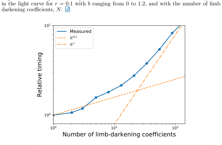
The central claim, stated on the paper's own terms, is that when the specific intensity is a polynomial in the elevation coordinate z, the observed flux factorizes as F = I0 s^T A u, where u lists the limb-darkening coefficients, A is a fixed change-of-basis matrix from those coefficients to a Green's basis, and s is a solution vector depending only on the radius ratio r and impact parameter b. The uniform, linear, and quadratic terms s0, s1, and s2 are given in stabilized form, and every higher-order term sn is obtained by reducing the two-dimensional surface integral, via Green's theorem, to a line integral around the occulting body whose primitive integrals are linear combinations of recursively defined integrals Mn(r,b). The paper derives analytic partial derivatives of F with respect to r, b, and the limb-darkening coefficients, including small-impact-parameter expressions for the b-derivative that avoid division by b. The authors claim that these formulas evaluate at near-double precision across the parameter plane, with the documented caveat that precision degrades for very high polynomial order, roughly N = 25-30, because of cancellations among large alternating coefficients.

Load-bearing premise

If the two bodies are not effectively spherical with azimuthally symmetric, sharp-edged limb darkening, the closed-form model describes the idealized star rather than the actual observation.

Editorial extensions

If this is right

Transit fits can treat limb-darkening coefficients as free parameters at any integer polynomial order without resorting to numerical integration, which is what high-precision space photometry is expected to require.
The analytic derivatives make gradient-based optimization, Fisher-matrix forecasts, and Hamiltonian Markov Chain Monte Carlo sampling of transit parameters practical, since the gradient of the likelihood can be computed without finite differences.
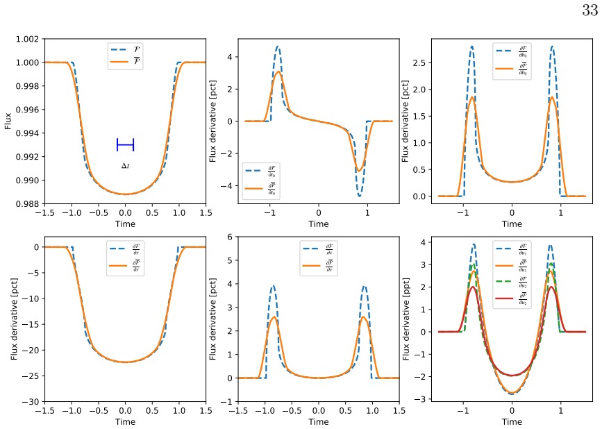
Finite-exposure light curves are handled by adaptive quadrature that splits exposures at contact points, so time-averaged fluxes and their derivatives are available without re-binning or losing contact information.
The same closed-form machinery applies to eclipsing binaries and multiple-star occultations when both stars are treated as spherical and limb-darkened.
The stabilized overlap-area formula removes the need for special series patches near first-to-fourth contact, so the same code paths work for the whole parameter range rather than switching to limiting expressions.

Reading between the lines

Editorial extensions of the paper, not claims the author makes directly.

Non-integer limb-darkening laws, such as the power-2 law, are not directly solvable by this machinery, but the paper's framework suggests a practical pipeline: fit a high-order polynomial to the non-linear profile once, then fit the few non-linear parameters against the precomputed polynomial coefficients.
The documented precision ceiling near N = 25-30 implies that 'arbitrary order' has a real double-precision limit; users wanting very flexible profiles should regularize the coefficients or stay in the Green's basis, where high-order terms contribute zero net unocculted flux and are easier to keep small.
The same recursion-and-line-integral scheme could be reused for other two-circle boundary problems, such as ring shadows or spot crossings, whenever the integrand is polynomial in z.
Because the region near r = b is now accurate, perturbative transit-timing-variation searches that expand timing shifts as a linear response to the derivative of the light curve can drop their interpolation patches and use the derivative directly.

Share X Bluesky LinkedIn Reddit HN

Signed reviews

No signed human review yet.

Editorial analysis

A structured set of objections, weighed in public.

Desk editor's note, referee report, and a circularity audit.

Desk Editor's Note

read the letter

You should know this paper for what it is: the first closed-form treatment of transit light curves for polynomial limb darkening of arbitrary integer order, complete with analytic derivatives for radius ratio, impact parameter, and limb-darkening coefficients. The derivation is explicit and self-contained, building on Green's theorem and a well-chosen Green's basis. The change-of-basis algebra checks out, the recursion relations for the M_n integrals are internally consistent, and the formulas reduce properly to the known uniform, linear, and quadratic cases. The authors also deliver a genuinely improved overlap-area formula for the uniform case, stabilized for the numerically nasty limits near contact, and they provide code in Julia, Python, IDL, and C++ with tests and reproduction scripts.

The validation is a real strength. They compare against 256-bit BigFloat arithmetic near the contact points and against Mandel & Agol (2002), Pál (2008), batman, and PyTransit. The speed benchmarks are credible: roughly 35-45% faster than EXOFAST, 70% faster than Pál's Fortran code, and 5-30x faster than the Giménez/PyTransit recursion for high orders. The self-reported precision degradation around N = 25-30 is disclosed, and the paper correctly cautions users to check high-order cases.

The soft spots are minor. The stress-test note is right: in Sec. 6 the higher-order s_n are defined only through the P integral and the k^2 branches, with no explicit special-case formulas for b = 0 or complete occultation (b < r - 1). Those regimes are physically important and the equations as written are not obviously valid there; the shipped code likely handles them, but the paper should say so. Also, the exposure-time-averaged derivatives are computed with adaptive Simpson quadrature rather than analytically; that is a practical choice, but it is a numerical step in an otherwise analytic paper. Neither issue affects the central claim.

On the physical side, the assumptions of spherical bodies, azimuthal symmetry, and sharp edges are explicitly stated in Sec. 12 and are standard across the field. They limit real-data applicability at JWST precision, but the paper acknowledges this and explains why a numerically stable ideal model still matters for fitting and gradient-based inference.

This is a useful and reproducible methods paper. The target audience is anyone fitting transits or eclipses with high-precision photometry, especially JWST-era users who want fast gradients for Hamiltonian MCMC or Fisher information. I would cite it and bring it to a reading group. It deserves a serious referee: the derivation is original, the validation is thorough, and the code is a genuine community resource.

Referee Report

2 major / 4 minor

Summary. This paper derives closed-form analytic expressions for the flux of a spherical star occulted by a circular, sharp-edged body, for limb-darkening profiles that are polynomials in the stellar elevation of arbitrary integer order. The flux is expressed as F = I0 s^T A u, where A is a fixed change-of-basis matrix, u contains the limb-darkening coefficients, and the solution vector s is computed by Green's theorem as a line integral plus recursion relations for the integrals M_n. The authors also derive analytic derivatives with respect to the radius ratio, impact parameter, and limb-darkening coefficients, and they compute exposure-time-averaged light-curve derivatives using adaptive Simpson quadrature. The paper validates the expressions against 256-bit BigFloat arithmetic and against Mandel & Agol (2002), Pál (2008), batman, and PyTransit, and it reports substantial improvements in numerical stability and speed.

Significance. If the derivation is correct, this is a substantial methodological contribution. The central construction is parameter-free in the sense that no fitted constants enter; the formulas follow from geometry and calculus, and the claims are supported by machine-checked derivations, reproducible code in multiple languages, and independent numerical benchmarks. The stability improvements near contact points and the availability of analytic derivatives are directly useful for gradient-based inference, Fisher-matrix calculations, and high-precision JWST-era transit modeling. The limitations imposed by the spherical, azimuthally symmetric, sharp-edged assumptions are disclosed in Section 12 and are standard for the field. The main gap I find is not in the core derivation but in the treatment of special geometric limits for the higher-order terms.

major comments (2)

[§6, Eqs. (71)-(78)]
[§5, Eqs. (53)-(56)]

minor comments (4)

[§3.1]
[Table 1]
[§12]
[§9-10]

Circularity Check

0 steps flagged · score 0.0 of 10

No significant circularity: the analytic derivation is self-contained and independently benchmarked.

full rationale

The derivation is self-contained. The central result F = I0 s^T A u (Eq. 100) follows directly from inserting the polynomial limb-darkening law into the surface integral (Eq. 7), applying the two explicitly derived change-of-basis operations (Eqs. 10-18), and reducing the surface integral to the line integral P(G_n) via Green's theorem (Eqs. 58-73). No fitted parameter is renamed as a prediction: the solution vector s_n is computed analytically from geometry, the normalization constant I0 is fixed by the unocculted-flux integral (Eqs. 23-28), and the derivatives (Eqs. 93-98) are obtained by differentiating the same analytic expressions. The Green's basis is derived within the paper (Eqs. 60-63) rather than imported as an unverified ansatz. Citations to Luger et al. (2019a,b) supply notation and a shared technique, but the load-bearing mathematical content is re-derived here, so the self-citation is not circular. Accuracy claims are checked against independent external codes (Mandel & Agol 2002, Pál 2008, batman, PyTransit) and against high-precision BigFloat arithmetic, and the comparisons do not depend on parameters fitted by this paper. The disclosed limitations in Sec. 12 (spherical bodies, azimuthal symmetry, sharp edges) and Sec. 10.1 (precision loss for N > 25) are explicit physical idealizations and numerical caveats, not circular inputs. No step of the derivation reduces, by construction or by definition, to its own inputs.

Assumptions & free parameters 3 free parameters · 5 assumptions · 0 invented entities

The central derivation has no fitted physical constants. The listed free parameters are numerical implementation choices (small-b cutoff, series truncation, integration tolerance). Standard mathematical tools and the explicit physical assumptions from §12 support the claim.

free parameters (3)

bc = 1e-3
Small-impact-parameter cutoff used to switch to the alternative expression for dP/db (Eq. 84). Chosen by hand for numerical stability, not derived.
jmax = 100
Truncation of the series expansions for M_n and N_n (Eqs. 81, 89). Set to 100 with a tolerance criterion; affects accuracy at high order.
epsilon_tol = 10^-4 to 10^-14
User-specified tolerance for adaptive Simpson time-integration of exposure-averaged light curves. The achieved precision scales roughly with 10 times this tolerance.

assumptions (5)

standard math Green's theorem reduces the surface integral to a line integral over the occultor and occulted-body boundaries.
Used in §6 to derive the P and Q primitive integrals.
standard math Complete elliptic integrals K, E, and Pi, and the Bulirsch cel function, can be evaluated accurately via Bartky recursion.
Relied on throughout §4-6 for linear and higher-order terms; numerical accuracy depends on this.
standard math The binomial expansion correctly transforms the (1-mu)^n limb-darkening basis to the polynomial and Green's bases.
Used in Eqs. (10)-(18) to construct the change-of-basis matrices.
domain assumption Stars and occultors are spherical with sharp edges, limb darkening is azimuthally symmetric, and refraction and relativistic effects are negligible.
Stated in §12; if violated, the model is not exact for real observations.
domain assumption The limb-darkening profile is exactly a polynomial in (1-mu) of finite integer order N.
This is the model in Eq. (3); real stellar profiles are not exactly polynomial but can be approximated.

how reviews work

0 comments

Cite this review

Pith. "Pith review of Analytic Planetary Transit Light Curves and Derivatives for Stars with Polynomial Limb Darkening." pith.science (2026). https://pith.science/paper/PLPCBM3M

@misc{pith2026190803222,
  author       = {Pith},
  title        = {Pith review of: Analytic Planetary Transit Light Curves and Derivatives for Stars with Polynomial Limb Darkening},
  year         = {2026},
  howpublished = {\url{https://pith.science/paper/PLPCBM3M}},
  note         = {Machine review of arXiv:1908.03222}
}

read the original abstract

We derive analytic, closed-form solutions for the light curve of a planet transiting a star with a limb darkening profile which is a polynomial function of the stellar elevation, up to arbitrary integer order. We provide improved analytic expressions for the uniform, linear, and quadratic limb-darkened cases, as well as novel expressions for higher order integer powers of limb darkening. The formulae are crafted to be numerically stable over the expected range of usage. We additionally present analytic formulae for the partial derivatives of instantaneous flux with respect to the radius ratio, impact parameter, and limb darkening coefficients. These expressions are rapid to evaluate, and compare quite favorably in speed and accuracy to existing transit light curve codes. We also use these expressions to numerically compute the first partial derivatives of exposure-time averaged transit light curves with respect to all model parameters. An additional application is modeling eclipsing binary or eclipsing multiple star systems in cases where the stars may be treated as spherically symmetric. We provide code which implements these formulae in C++, Python, IDL, and Julia, with tests and examples of usage.

Figures

Figures reproduced from arXiv: 1908.03222 by the authors.

**Figure 1.** The area of overlap of two circles can be computed as the sum of the area of the sectors formed by the centers of each circle and the boundary between the points of intersection, minus the area of the kite-shaped region formed by the centers of the circles and the intersection points. 6 Evaluation of the transit light curve of a uniformly bright star, I(µ) = 1, amounts to computing the area of overlap of two disks (… view at source ↗

**Figure 2.** Precision of formulae for the area of overlap of two circles with radius ratio r. Plotted are the regions near b = 1 − r (second and third points of contact) and b = 1 + r (first and fourth points of contact) for the standard formula (Equation 29, blue) and our new formula (Equation 33, orange dots). The high-precision calculation is shown in green dashed for comparison; this is limited by the conversion of the resu… view at source ↗

**Figure 3.** The flux of a linearly limb-darkened star being eclipsed, F = 3 2π s1(r, b), with u1 = 1 (all other un zero), for which I0 = 3/(2π). In the limit b > r + 1, no eclipse occurs, so F = 1. For b < r − 1, the star is completely eclipsed and F = 0. In the limits b = r and b = 1 − r, special expressions must be used. 6 0.00 0.25 0.50 0.75 1.00 1.25 1.50 1.75 2.00 1.2 1.4 1.6 1.8 2.0 1 1(r=b± , b) r=b r=b+ r=b 0.00 0.25 0.… view at source ↗

Figures from the paper (15 more)

**Figure 4.** Figure 4: The accuracy of s1(r, b) near b = r (left panels) and b = 1 − r (right panels) for = 10−8 . The x-axes are impact parameter b, while the y axes in the top panels show s1(r, b), with r given in the legend of each panel. The middle panels plot the difference (s1(b ± ,…

**Figure 5.** Figure 5: The numerical error in computing the flux of an eclipsed, linearly limb-darkened star (u1 = 1) using the equations in Mandel & Agol (2002). 6 0.0 0.5 1.0 1.5 2.0 Impact parameter 0.00 0.25 0.50 0.75 1.00 1.25 1.50 1.75 2.00 Radius ratio r=1+b r=b r=b 1 r=1 b 1.5×10 15 …

**Figure 6.** Figure 6: The numerical error in computing the flux of an eclipsed, linearly limb-darkened star (u1 = 1) using the s1(r, b) formalism introduced in this paper. Compare to [PITH_FULL_IMAGE:figures/full_fig_p020_6.png]

**Figure 7.** Figure 7: Comparison of the normalized flux and its derivatives with and without timeintegration (see solid and dashed lines, respectively). The integration time, ∆t = 0.3, is indicated in the upper left panel with a horizontal blue line. The derivatives are computed with respe…

**Figure 8.** Figure 8: Precision achieved for the time-integrated flux (minus one) versus the average number of evaluations per exposure. The colored lines show the precision achieved for F(t)−1 and for each of the derivatives. For comparison, the dotted line shows 10 times the tolerance, t…

**Figure 9.** Figure 9: Comparison of the non-linear limb darkening with polynomial fits of various orders. 6 non-linear limb darkening light curves in the code of Mandel & Agol (2002), and it is analogous to the approach taken by Kreidberg (2015) for computing models with arbitrary limb dark…

**Figure 10.** Figure 10: Scaling of the computation time in seconds with the number of data points in the light curve for r = 0.1 with b ranging from 0 to 1.2, and with the number of limb darkening coefficients, N. 6 10 0 10 1 10 2 Number of limb-darkening coefficients 10 0 10 1 Relative timi…

**Figure 11.** Figure 11: Scaling of the computation time with the number of limb darkening coeffients, N. The y-axis scales the timing with respect to the timing for a single limb darkening coefficient. 6 parameters, we carried out nine measurements of the timing, and we use the median of the…

**Figure 12.** Figure 12: Values of the gn vector versus n for N = 20 and for uniform values of un = 1/20. 6 core without multi-threading or interpolation over a pre-computed grid, which is an option in some codes. 11.1. Comparison with Mandel & Agol (2002) For uniform, linear or quadratic lim…

**Figure 13.** Figure 13: The fractional error on a light curve computed as a function of N, the order of the limb-darkening. The dotted points show the results of the maximum fractional error (relative to the depth of the transit) for ten different random realizations of the un limb-darkening…

**Figure 14.** Figure 14: Comparison of Mandel & Agol (2002) with Agol, Luger, & Foreman-Mackey (2019). 6 precision for the computation, with errors reaching as much as a few ×10−8 for the flux and the derivatives with respect to the limb darkening parameters. One possible origin for this diff…

**Figure 15.** Figure 15: Comparison of Pál (2008) with Agol, Luger, & Foreman-Mackey (2019). The coefficients are u1 = 0.2 and u2 = 0.3. 6 [PITH_FULL_IMAGE:figures/full_fig_p043_15.png]

**Figure 16.** Figure 16: Comparison of Kreidberg (2015) (orange) with Agol, Luger, & ForemanMackey (2019) (Julia implementation in blue and starry implementation in green) for a transit across a quadratically limb-darkened star. Also shown are points corresponding to the computation using Py…

**Figure 17.** Figure 17: Similar to [PITH_FULL_IMAGE:figures/full_fig_p044_17.png]

**Figure 18.** Figure 18: Comparison of the algorithm presented in this work (blue and green points) to that of Giménez (2006) for the computation of a transit across a star with polynomial limb darkening, as implemented in the PyTransit package (Parviainen 2015) (purple points), as a function…

Discussion (0). Continue with ORCID to comment.

Forward citations

Cited by 1 Pith paper

Reviewed papers in the Pith corpus that reference this work. Sorted by Pith novelty score. Full citation record

The ExoTETHyS package: Tools for Exoplanetary Transits around Host Stars
astro-ph.EP 2019-08 conditional novelty 6.0 of 10

A new weighted fitting algorithm for stellar limb-darkening coefficients reduces transit light-curve model residuals to below 10 parts per million, and an exact light-curve generator avoids limb-darkening laws entirely.

Reference graph

Works this paper leans on

13 extracted references · 7 canonical work pages · cited by 1 Pith paper

[1]

In Equation (7),λ3 and λ4 should have 2k→ 2p in arguments of the elliptic integrals

work page
[2]

In Equation (7),λ5 should have− 2 3Θ(p− 1/2) at the end

work page
[3]

For Case 11 in Table 1,ηd should be 1/2, not 1, andλd should be zero, not

work page
[4]

The casez = 1−p is missing forz <p (as pointed out by Pal 2008)

work page 2008
[5]

With the exception of 3, none of these errors aﬀected the publicly available code

There is aπ missing in the denominator of the second term on the right hand side of Equation (8). With the exception of 3, none of these errors aﬀected the publicly available code. B. DERIVATIVES OF GENERAL COMPLETE ELLIPTIC INTEGRAL In this appendix, we give the derivatives ofcel with respect to the input parameters. ∂cel(kc,p,a,b ) ∂kc = −kc p−k2 c [ ce...

work page 2002
[11]

This typo was discussed in Eastman et al

This mistake aﬀects the code, but it is never encountered for planets that transit main-sequence stars sincep< 1. This typo was discussed in Eastman et al. (2013)

work page 2013
[123]

1467-9868.2010.00765.x Goldberg, D

https://doi.org/10.1111/j. 1467-9868.2010.00765.x Goldberg, D. 1991, ACM Computing Surveys, 23, 5. https://doi.org/10.1145/103162.103163 Hastings, C. 1955, Approximations for digital computers„ Princeton, N.J.: Princeton University Press Haswell, C. A. 2010, Transiting Exoplanets Hayek, W., et al. 2012, Astronomy & Astrophysics, 539, A102. https: //doi.or...

arXiv 2010
[385]

Circle-Circle Intersection

https://doi.org/10.1086/141972 Sanchis-Ojeda, R., & Winn, J. N. 2011, The Astrophysical Journal, 743, 61. https: //doi.org/10.1088/0004-637x/743/1/61 Seager, S., & Deming, D. 2010, Annual Review of Astronomy and Astrophysics, 48, 631. https://doi.org/10.1146/ annurev-astro-081309-130837 Seager, S., & Hui, L. 2002, The Astrophysical Journal, 574, 1004. htt...

work page doi:10.1086/141972 2002

Show all 13 references

[505]

2017, The Astronomical Journal, 154, 220

https://doi.org/10.1086/500802 Foreman-Mackey, D., et al. 2017, The Astronomical Journal, 154, 220. https: //doi.org/10.3847/1538-3881/aa9332 Giménez, A. 2006, Astronomy & Astrophysics, 450, 1231. https: //doi.org/10.1051/0004-6361:20054445 Girolami, M., & Calderhead, B. 2011,...

2017 doi
[567]

1365-2966.2005.08922.x Alonso, R

https://doi.org/10.1111/j. 1365-2966.2005.08922.x Alonso, R. 2018, in Handbook of Exoplanets (Springer International Publishing), 1441–1467. https://doi.org/ 10.1007/978-3-319-55333-7_40 Barnes, J. W. 2009, The Astrophysical Journal, 705, 683. https: //doi.org/10.1088/0004-637...

2005
[1193]

1938, Reviews of Modern Physics, 10, 264

https://doi.org/10.1086/425067 Bartky, W. 1938, Reviews of Modern Physics, 10, 264. https: //doi.org/10.1103/revmodphys.10.264 Beichman, C., et al. 2014, Publications of the Astronomical Society of the Paciﬁc, 126, 1134. https://doi.org/10.1086/679566 Betancourt, M. 2017, arXi...

1938 arXiv
[1515]

1365-2966.2011.18122.x Hui, L., & Seager, S

https://doi.org/10.1111/j. 1365-2966.2011.18122.x Hui, L., & Seager, S. 2002, The Astrophysical Journal, 572, 540. https://doi.org/10.1086/340017 52 Kahan, W. 2000, Technical report, University of California, Berkeley Kipping, D. M. 2010, Monthly Notices of the Royal Astronomi...

2011
[1758]

1365-2966.2010.17242.x —

https://doi.org/10.1111/j. 1365-2966.2010.17242.x —. 2013, Monthly Notices of the Royal Astronomical Society, 435, 2152. https://doi.org/10.1093/mnras/stt1435 Kopal, Z. 1950, Harvard College Observatory Circular, 454, 1 Kreidberg, L. 2015, PASP, 127, 1161 Kuncir, G. F. 1962, C...

2010

Pith tools

Reviewed August 14, 2026 · model on record in the stance chip above.

[1] [1]

In Equation (7),λ3 and λ4 should have 2k→ 2p in arguments of the elliptic integrals

work page

[2] [2]

In Equation (7),λ5 should have− 2 3Θ(p− 1/2) at the end

work page

[3] [3]

For Case 11 in Table 1,ηd should be 1/2, not 1, andλd should be zero, not

work page

[4] [4]

The casez = 1−p is missing forz <p (as pointed out by Pal 2008)

work page 2008

[5] [5]

With the exception of 3, none of these errors aﬀected the publicly available code

There is aπ missing in the denominator of the second term on the right hand side of Equation (8). With the exception of 3, none of these errors aﬀected the publicly available code. B. DERIVATIVES OF GENERAL COMPLETE ELLIPTIC INTEGRAL In this appendix, we give the derivatives ofcel with respect to the input parameters. ∂cel(kc,p,a,b ) ∂kc = −kc p−k2 c [ ce...

work page 2002

[6] [11]

This typo was discussed in Eastman et al

This mistake aﬀects the code, but it is never encountered for planets that transit main-sequence stars sincep< 1. This typo was discussed in Eastman et al. (2013)

work page 2013

[7] [123]

1467-9868.2010.00765.x Goldberg, D

https://doi.org/10.1111/j. 1467-9868.2010.00765.x Goldberg, D. 1991, ACM Computing Surveys, 23, 5. https://doi.org/10.1145/103162.103163 Hastings, C. 1955, Approximations for digital computers„ Princeton, N.J.: Princeton University Press Haswell, C. A. 2010, Transiting Exoplanets Hayek, W., et al. 2012, Astronomy & Astrophysics, 539, A102. https: //doi.or...

arXiv 2010

[8] [385]

Circle-Circle Intersection

https://doi.org/10.1086/141972 Sanchis-Ojeda, R., & Winn, J. N. 2011, The Astrophysical Journal, 743, 61. https: //doi.org/10.1088/0004-637x/743/1/61 Seager, S., & Deming, D. 2010, Annual Review of Astronomy and Astrophysics, 48, 631. https://doi.org/10.1146/ annurev-astro-081309-130837 Seager, S., & Hui, L. 2002, The Astrophysical Journal, 574, 1004. htt...

work page doi:10.1086/141972 2002