REVIEW 3 major objections 6 minor 51 references
Recurrent U-net: Deep learning to predict daily summertime ozone in the United States
T0 review · 3 major / 6 minor · reviewed 2026-08-14 · deepseek-v4-flash
Pith's one-line read The paper claims that a recurrent U-net trained on meteorological reanalysis fields and sector-specific NOx emissions predicts daily summertime MDA8 ozone across the United States with r2 = 0.83, and that using the model to test post-2010…
desk verdict A solid out-of-sample ozone prediction study with a policy-relevant emission-trend claim that is more fragile than the abstract implies, because the trend test scales emissions by a single national factor. read the letter →
The pith
A machine-rendered reading of the paper's core claim, the machinery that carries it, and where it could break.
The reading
What carries the argument
The load-bearing mechanism is the recurrent U-net architecture: a fully convolutional encoder that compresses 13 input channels (six ERA-Interim meteorological fields and seven CEDS NOx emission sectors) into a latent space, three stacked long short-term memory (LSTM) cells that carry temporal state across days and years, and a transposed-convolution decoder with skip connections that restore spatial detail. The model is trained to minimize the mean squared error between predicted and observed MDA8 ozone in AQS-observed grid boxes. The emission-trend evaluation then uses Equation (3), $E_i^m = E_i^{\mathrm{CEDS}} \cdot \beta_m$, which scales every CEDS monthly emission field by a single national annual factor $\beta_m$ derived from each inventory trend, so the learned meteorological-ozone relationships stay fixed while only the emission trend changes.
What would settle it
A concrete test would be to rerun the 2010-2016 predictions using the actual spatially and sectorally resolved EPA emission trends instead of a uniform national scaling factor; if the negative bias in predicted MDA8 ozone disappears or becomes comparable to the top-down trends, the conclusion that the EPA inventory overestimates NOx reductions would be undercut. Alternatively, an independent chemical transport simulation using EPA emissions that reproduces observed MDA8 ozone without bias over the same period would contradict the paper's claim.
Extended reading notes
Core claim
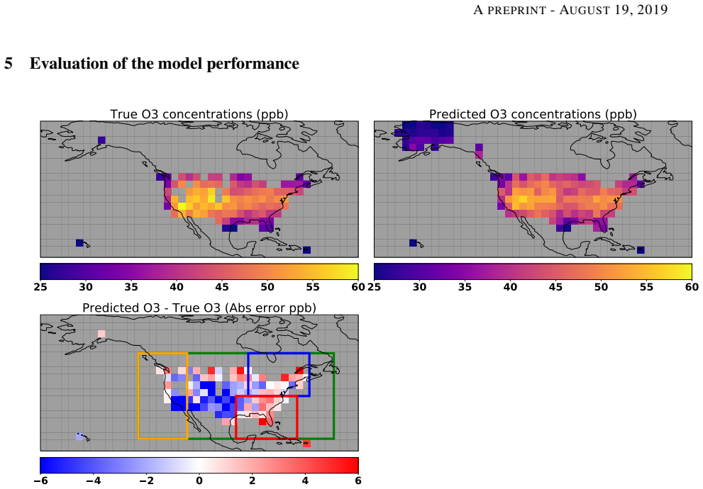
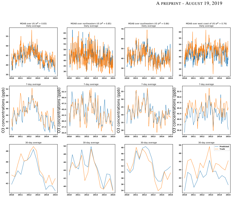
The central claim is that a recurrent U-net, without any explicit representation of ozone photochemistry, captures the daily, seasonal, and interannual variability of US summer MDA8 ozone well enough to serve both as a prediction system and as a diagnostic of emission trends. On the withheld 2010-2014 test period the model achieves r2 = 0.83 over the contiguous United States, with regionally high skill in the East and West Coast (r2 about 0.75-0.86) and weaker skill in the Intermountain West (r2 about 0.4). When the CEDS emissions input is rescaled by annual national factors representing the EPA, AQS NO2, TCR-2, and Jiang et al. trends, the EPA trend yields the largest negative mean error (-2.18 ppb) for 2010-2016, while TCR-2 gives the smallest; in urban boxes the AQS NO2 trend performs best, and in rural boxes the top-down trends perform best. The authors interpret these patterns as evidence that the top-down trends reflect both anthropogenic and background NOx changes, and that the EPA bottom-up inventory is overestimating post-2010 NOx reductions.
Load-bearing premise
The trend evaluation assumes that the CEDS spatial and sectoral distribution of NOx emissions is correct and that each inventory's trend can be represented by a single national annual scaling factor applied uniformly across the United States, while the model's learned ozone-NOx sensitivity is extrapolated to emission levels and spatial patterns beyond its 1980-2009 training distribution.
Editorial extensions
If this is right
- If the model's skill holds, deep learning offers an operational alternative to chemical transport models for daily ozone prediction, avoiding the 10-20 ppb summertime overestimate those models typically show in the eastern United States.
- The model can produce ozone predictions at every grid box even where no AQS monitor exists, extending air-quality information into observation-sparse regions.
- The feature-map analysis implies the trained model has learned physically meaningful teleconnections (Pacific and Atlantic sea surface temperature and sea-level pressure patterns) and that power, industry, and transportation NOx sectors drive ozone predictability.
- If the EPA trend is indeed overestimating NOx reductions, then air-quality management based on bottom-up inventories has been underestimating the remaining NOx control burden since 2010.
Reading between the lines
- Our inference: since the model's skill depends on the 1980-2009 training distribution, its credibility beyond 2016 rests on continued validation against recent AQS data; retraining through 2014 and testing on 2015-2020 would clarify how far the learned NOx-ozone sensitivity extrapolates.
- Our inference: the single national scaling factor in Equation (3) is a coarse lens; regional or sector-specific rescaling of emissions would likely sharpen the urban/rural signal already visible in the paper's error statistics.
- Our inference: the same architecture could be applied to forecast ozone using predicted meteorological fields from operational weather models, and transferred to other pollutants such as PM2.5, which the paper notes as future potential but does not test.
Signed reviews
Editorial analysis
A structured set of objections, weighed in public.
Referee Report
Summary. The manuscript presents a hybrid deep learning model, a recurrent U-net (convolutional encoder-decoder with stacked LSTM cells and skip connections), to predict daily June-July-August (JJA) maximum daily 8-hour average (MDA8) surface ozone over the contiguous United States. Predictors are ERA-Interim meteorological fields (MSLP, 500-hPa geopotential, downward shortwave radiation, SST, 2-m temperature, 2-m dew point) and monthly mean sector-resolved NOx emissions from the CEDS inventory. The model is trained on EPA AQS ozone measurements from 1980-2009 (with the last 15% used for validation) and tested on 2010-2014. The authors report a CONUS test-period r2 of 0.83 and a mean error of -1.14 ± 1.94 ppb, with high skill in the eastern US and West Coast but lower skill in the Intermountain West. Feature-map analyses are used to argue that the model captures teleconnections. In the second part, the trained model is used to evaluate NOx emission trends after 2010 by scaling CEDS emissions with annual national factors derived from the EPA bottom-up inventory, AQS surface NO2 observations, and two satellite-based top-down inventories (TCR-2 and Jiang et al.). The EPA trend produces the largest negative bias in predicted MDA8 ozone, whereas the TCR-2 trend gives the best overall agreement; urban/rural disaggregation shows AQS best in urban areas and top-down trends best in rural areas.
Significance. If the central claims hold, the paper makes two contributions: (1) a demonstration that a deep recurrent convolutional model can provide high-skill, temporally out-of-sample predictions of daily summertime surface ozone, with skill well above the reported performance of conventional chemical transport models; and (2) a novel empirical framework for evaluating NOx emission inventories using observed ozone alone. The design has real strengths: the temporal train/test split is clean, the metrics are clearly defined, the appendices provide the network equations and a retraining sensitivity experiment, and the trend evaluation compares external inventories rather than re-fitting to the test target. However, the second contribution is currently weakened by a load-bearing modeling assumption in the emission-trend comparison, so the headline policy conclusion is not yet established to the standard that the paper claims.
major comments (3)
- [§6, Eq. (3)] Equation (3) scales every CEDS NOx emission field by a single national annual factor β_m for each inventory, so the evaluation implicitly assumes both that the CEDS spatial distribution and sectoral split are correct for 2010-2016 and that the relative emission trend is uniform across all grid boxes and all seven sectors. Neither assumption is tested. The paper's own Table 3 indicates that the optimal trend differs between urban and rural regions (AQS NO2 best in urban, TCR-2 best in rural), which is difficult to reconcile with a scalar national trend. Because ozone production responds nonlinearly to NOx and the sensitivity regime varies spatially (Section 5 notes that urban cores can be VOC-limited), the CONUS mean errors in Table 2 do not provide a clean test of 'EPA vs TCR-2' emission trends; they test scalar versions of those trends imposed on the CEDS spatial pattern. The conclusion that the EPA inventory overestimates NOx reductions after 2010 is therefore not established by this experiment. I recommend testing regionally or sectorally varying scaling factors, or directly comparing model predictions driven by the full spatial and sectoral patterns of each inventory.
- [§6, Appendix E] Appendix E retrains the model on 1980-2005 and evaluates 2005-2016, which is a useful robustness check that partly mitigates concerns about extrapolation beyond the original training period. However, the same scalar scaling in Eq. (3) is applied, so the experiment does not address the spatial-uniformity issue. In addition, for 2010-2016 the EPA-scaled emissions fall below the lowest NOx levels seen in the 1980-2009 training data, so the model is being asked to predict ozone in an emission regime it has never seen; the lower r2 values in Table 5 (0.72-0.75) relative to Table 2 (0.79-0.81) are consistent with this. The agreement among all trends in 2005-2009 (Table 4) is reassuring, but it does not validate the post-2010 extrapolation. Please add an analysis that constrains the emission perturbation to the training range, or otherwise quantify the model's sensitivity to out-of-distribution emission inputs.
- [§6, Tables 2-5] The ranking of emission trends (e.g., 'TCR-2 produced the smallest error', 'EPA resulted in the largest negative bias') is not accompanied by any statistical significance test. The reported ±1σ values are the standard deviations of the daily grid-box errors, not uncertainties of the mean, so the reader cannot judge whether the differences among scenarios (e.g., TCR-2 mean error 0.55 ppb vs AQS -1.06 ppb) are meaningful or simply sampling noise. Please provide paired significance tests or bootstrap confidence intervals for the mean-error comparisons, accounting for spatial and temporal autocorrelation.
minor comments (6)
- [§4, Eq. (2)] Equation (2) is described as 'the square of the Pearson correlation coefficient,' but the formula shown is the coefficient of determination (1 - SS_res/SS_tot), which is not generally equal to the squared Pearson correlation for arbitrary predictions; please use consistent terminology and notation, e.g., R².
- [Figures 3, 4, 6] The r² values printed in the panel titles are not labelled by averaging window; please specify whether they refer to daily, 7-day, or 30-day means, since the three rows of each figure display different temporal aggregates.
- [§3] The manuscript states that ozone data are aggregated to 3°×3° grid boxes while the meteorological fields are at 1.5°; it is not explained how the model output grid and the observational grid are reconciled in the loss function and in the evaluation metrics.
- [§5, Appendix D] There are several typographical errors: 'The model account for 96%' should be 'accounts'; 'wherer2≈ 0.4' should be 'where r2≈ 0.4'; 'Fig. 9 the the feature maps' has a duplicated 'the'; and Section 7 has 'relative to tat from' which should read 'to that from'.
- [§6, Table 3] The urban/rural classification is defined by a NOx emission threshold of 1×10^11 molec cm^-2 s^-1 following Li and Wang; please specify whether this threshold is applied to the CEDS emissions, the scaled emissions, or another inventory, and how it is mapped to the 3° grid boxes.
- [§5] The statement that the deep learning model 'captures the physical and chemical mechanisms' is stronger than what an empirical model can establish; a more precise phrasing such as 'captures statistical relationships consistent with known mechanisms' would be appropriate.
Circularity Check
No significant circularity: predictions are genuine temporal out-of-sample forecasts and the inventory comparison is not encoded in the training target.
full rationale
The central predictive claim is evaluated on 2010-2014 AQS MDA8 ozone, which was not used for training (1980-2009), so the r2=0.83 skill score is not a fitted artifact. The NOx-trend evaluation in Section 6 uses Eq. (3) to scale the CEDS emission fields by annual factors derived from four independent trend products (EPA bottom-up, AQS NO2 observations, Jiang et al., TCR-2). None of these scaling factors is fit to the AQS MDA8 ozone used as the evaluation target, and the model has no access to the 2010-2016 ozone in training. The Jiang et al. and TCR-2 inventories involve overlapping authors, and TCR-2 was preprint/in-prep at the time, but they are external data products based on satellite retrievals and data assimilation, not on the present model's fitted values; therefore their use is not a self-citation chain. The assumption that a single national beta captures spatially uniform emission trends is a modeling limitation and a correctness risk, but it is not a circular reduction of the conclusion to its inputs. The Appendix E retraining experiment provides an additional out-of-sample check. No equation reduces to a fitted target by construction.
Assumptions & free parameters
free parameters (5)
- Neural network weights and biases (55 million trainable parameters) =
Not shipped
- Training hyperparameters (learning rate, batch size, number of epochs, early stopping, normalization) =
Not reported
- Architecture hyperparameters (number of filters, kernel sizes, LSTM hidden state size, decoder depths) =
Not fully specified
- Validation split fraction =
15% of training data
- Urban/rural NOx emission threshold =
1e11 molec cm-2 s-1
assumptions (5)
- domain assumption AQS MDA8 observations aggregated to 3x3 grid boxes represent true grid-box mean surface ozone.
- domain assumption ERA-Interim reanalysis fields are sufficiently accurate as ozone predictors.
- domain assumption CEDS inventory gives the correct spatial distribution and base-year magnitude of NOx emissions.
- domain assumption The trained model's ozone response to NOx emission scaling is a valid surrogate for real atmospheric response in 2010-2016.
- domain assumption Ozone photochemistry can be represented by the chosen 13 predictors without explicit VOC emissions or chemical mechanism.
Cite this review
Pith. "Pith review of Recurrent U-net: Deep learning to predict daily summertime ozone in the United States." pith.science (2026). https://pith.science/paper/POFZMVU3
@misc{pith2026190805841,
  author       = {Pith},
  title        = {Pith review of: Recurrent U-net: Deep learning to predict daily summertime ozone in the United States},
  year         = {2026},
  howpublished = {\url{https://pith.science/paper/POFZMVU3}},
  note         = {Machine review of arXiv:1908.05841}
}
abstract
We use a hybrid deep learning model to predict June-July-August (JJA) daily maximum 8-h average (MDA8) surface ozone concentrations in the US. A set of meteorological fields from the ERA-Interim reanalysis as well as monthly mean NO$_x$ emissions from the Community Emissions Data System (CEDS) inventory are selected as predictors. Ozone measurements from the US Environmental Protection Agency (EPA) Air Quality System (AQS) from 1980 to 2009 are used to train the model, whereas data from 2010 to 2014 are used to evaluate the performance of the model. The model captures well daily, seasonal and interannual variability in MDA8 ozone across the US. Feature maps show that the model captures teleconnections between MDA8 ozone and the meteorological fields, which are responsible for driving the ozone dynamics. We used the model to evaluate recent trends in NO$_x$ emissions in the US and found that the trend in the EPA emission inventory produced the largest negative bias in MDA8 ozone between 2010-2016. The top-down emission trends from the Tropospheric Chemistry Reanalysis (TCR-2), which is based on satellite observations, produced predictions in best agreement with observations. In urban regions, the trend in AQS NO$_2$ observations provided ozone predictions in agreement with observations, whereas in rural regions the satellite-derived trends produced the best agreement. In both rural and urban regions the EPA trend resulted in the largest negative bias in predicted ozone. Our results suggest that the EPA inventory is overestimating the reductions in NO$_x$ emissions and that the satellite-derived trend reflects the influence of reductions in NO$_x$ emissions as well as changes in background NO$_x$. Our results demonstrate the significantly greater predictive capability that the deep learning model provides over conventional atmospheric chemical transport models for air quality analyses.
Figures


Figures from the paper (9 more)


Reference graph
Works this paper leans on
-
[1]
Almaraz, M., E. Bai, C. Wang, J. Trousdell, S. Conley, I. Faloona, B. Z. Houlton (2018) Agriculture is a major source of NOx pollution in California. Sci. Adv. 4, eaao3477
work page 2018
-
[2]
Benediktsson, J. A., Swain, P. H. & Ersoy, O. K. Neural network approaches versus statistical methods in classifcation of multisource remote sensing data. IEEE Trans. Geosci. Remote Sens. 28, 540–552 (1990)
work page 1990
-
[3]
Bloomer BJ, Stehr JW, Piety CA, Salawitch RJ, Dickerson RR (2009) Observed relationships of ozone air pollution with temperature and emissions. Geophys Res Lett 36:L09803
work page 2009
-
[4]
Geophys Res Lett 42(9):3414-3420
Bond NA, Cronin MF, Freeland H, Mantua N (2015) Causes and impacts of the 2014 warm anomaly in the NE Pacific. Geophys Res Lett 42(9):3414-3420
work page 2015
-
[5]
Camps-Valls, G., Tuia, D., Bruzzone, L. & Benediktsson, J. A. Advances in hyperspectral image classifcation: Earth monitoring with statistical learning methods. IEEE Signal Process. Mag. 31, 45–54 (2014)
work page 2014
-
[6]
Cooper OR, Gao RS, Tarasick D, Leblanc T, Sweeney C (2012) Long-term ozone trends at rural ozone monitoring sites across the United States, 1990–2010. J Geophys Res 117:D22307
work page 2012
-
[7]
Dee, D. P., et al. (2011), The ERA-Interim reanalysis: configuration and performance of the data assimilation system. Q.J.R. Meteorol. Soc., 137: 553–597. doi: 10.1002/qj.828
doi:10.1002/qj.828 2011
-
[8]
Duncan, B. N., Yoshida, Y ., Olsen, J. R., Sillman, S., Martin, R. V ., Lamsal, L., . . . Crawford, J. H. (2010). Application of OMI observations to a space-based indicator of NOx and VOC controls on surface O3 formation. Atmospheric Environment, 44(18), 2213-2223. https://doi.org/10.1016/j.atmosenv.2010.03.010
Show all 51 references
-
[9]
(2009) Multimodel estimates of intercontinental sourcereceptor relationships for ozone pollution
Fiore AM, et al. (2009) Multimodel estimates of intercontinental sourcereceptor relationships for ozone pollution. J Geophys Res 114:D04301
2009
-
[10]
M., Naik, V ., and Leibensperger, E
Fiore, A. M., Naik, V ., and Leibensperger, E. M.: Air Quality and Climate Connections, J. Air Waste Manage., 65, 645–685, doi:10.1080/10962247.2015.1040526, 2015
2015
-
[11]
Atmos Environ 34(2):171–176
Gardner MW, Dorling SR (2000) Meteorologically adjusted trends in UK daily maximum surface ozone concen- trations. Atmos Environ 34(2):171–176
2000
-
[12]
Gill A (1980) Some simple solutions for heat-induced tropical circulation. Q. J. R. Meteorol Soc 106(449):447-462
1980
-
[13]
& Camps-Valls, G
Gomez-Chova, L., Tuia, D., Moser, G. & Camps-Valls, G. Multimodal classifcation of remote sensing images: a review and future directions. Proc. IEEE 103, 1560–1584 (2015)
2015
-
[14]
(2016) Deep Learning
Goodfellow I., et al. (2016) Deep Learning. MIT Press
2016
-
[15]
Digital selection and analogue amplification coexist in a cortex-inspired silicon circuit
Hahnloser, R.; Sarpeshkar, R.; Mahowald, M. A.; Douglas, R. J.; Seung, H. S. (2000). "Digital selection and analogue amplification coexist in a cortex-inspired silicon circuit". Nature. 405: 947–951. doi:10.1038/35016072
2000 doi
-
[16]
Long short-term memory
Hochreiter S., and Jürgen Schmidhuber (1997). "Long short-term memory". Neural Computation. 9 (8): 1735–1780. doi:10.1162/neco.1997.9.8.1735. PMID 9377276
1997 doi
-
[17]
Bengio, P
Hochreiter, S., Y . Bengio, P. Frasconi, and J. Schmidhuber. Gradient flow in recurrent nets: the difficulty of learning long-term dependencies. In S. C. Kremer and J. F. Kolen, editors, A Field Guide to Dynamical Recurrent Neural Networks. IEEE Press, 2001
2001
-
[18]
M., Smith, S
Hoesly, R. M., Smith, S. J., Feng, L., Klimont, Z., Janssens-Maenhout, G., Pitkanen, T., Seibert, J. J., Vu, L., Andres, R. J., Bolt, R. M., Bond, T. C., Dawidowski, L., Kholod, N., Kurokawa, J.-I., Li, M., Liu, L., Lu, Z., Moura, M. C. P., O’Rourke, P. R., and Zhang, Q.: Hist...
2018
-
[19]
Steinberger, R
Jaegle, L., L. Steinberger, R. V . Martin, K. Chance (2005) Global partitioning of NOx sources using satellite observations: Relative roles of fossil fuel combustion, biomass burning and soil emissions. Faraday Discuss. 130, 407-423
2005
-
[20]
Brian, W
Jiang, Z., M. Brian, W. Helen, W. John, M. Kazuyuki, Q. Zhen, D. K. Henze, D. B. A. Jones, A. F. Arellano, E. V . Fischer, L. Zhu, and K. F. Boersma. (2018). Unexpected slowdown of US pollutant emission reduction in the past decade. Proceedings of the National Academy of Scien...
2018 doi
-
[21]
M., Murray, L
Jin, X., Fiore, A. M., Murray, L. T., Valin, L. C., Lamsal, L. N., Duncan, B., . . . Tonnesen, G. S. (2017). Evaluating a space-based indicator of surface ozone-NOx-VOC sensitivity over midlatitude source regions and application to decadal trends. Journal of Geophysical Resear...
2017 doi
-
[22]
Proc Natl Acad Sci USA 111(40):14360-14365
Johnstone JA, Mantua NJ (2014) Atmospheric controls on northeast Pacific temperature variability and change, 1900-2012. Proc Natl Acad Sci USA 111(40):14360-14365. 20 A PREPRINT - AUGUST 19, 2019
2014
- [23]
-
[24]
Boser, J
LeCun,Y ., B. Boser, J. S. Denker, D. Henderson, R. E. Howard, W. Hubbard, L. D. Jackel, (1989). Backpropagation Applied to Handwritten Zip Code Recognition; AT&T Bell Laboratories
1989
-
[25]
C., Sengupta, S
Lee, J., Weger, R. C., Sengupta, S. K. & Welch, R. M. A neural network approach to cloud classifcation. IEEE Trans. Geosci. Remote Sens. 28, 846–855 (1990)
1990
-
[26]
Li, J., Wang, Y ., & Qu, H. (2019). Dependence of summertime surface ozone on NOx and VOC emissions over the United States: Peak time and value. Geophysical Research Letters, 46, 3540-3550. https://doi.org/10.1029/2018GL081823
2019 doi
-
[27]
and Wang, Y
Li, J. and Wang, Y . (2019), Inferring the anthropogenic NOx emission trend over the United States during 2003-2017 from satellite observations: Was there a flattening of the emission tend after the Great Recession?, Atmos. Chem. Phys. Discuss., https://doi.org/10.5194/acp-2019...
2019 doi
-
[28]
W., Cooper, O
Lin, M., Horowitz, L. W., Cooper, O. R., Tarasick, D., Conley, S., Iraci, L. T., Johnson, B., Leblanc, T., Petropavlovskikh, I., and Yates, E. L.: Revisiting the evidence of increasing springtime ozone mixing ratios in the free troposphere over western North America, Geophys. ...
-
[29]
Lin, M., A. M. Fiore, L. W. Horowitz, A. O. Langford, S. J. Oltmans, D. Tarasick, and H. E. Rieder (2015), Climate variability modulates western U.S. ozone air quality in spring via deep stratospheric intrusions, Nat. Commun., 6(7105), doi:10.1038/ncomms8105
2015 doi
-
[30]
W., Payton, R., Fiore, A
Lin, M., Horowitz, L. W., Payton, R., Fiore, A. M., and Tonnesen, G.: US surface ozone trends and extremes from 1980 to 2014: quantifying the roles of rising Asian emissions, domestic controls, wildfires, and climate, Atmos. Chem. Phys., 17, 2943-2970, https://doi.org/10.5194/a...
1980 doi
-
[31]
Liu, Y . et al. Application of deep convolutional neural networks for detecting extreme weather in climate datasets. In ABDA’16-International Conference on Advances in Big Data Analytics 81–88 https://arxiv.org/abs/1605.01156 (2016)
2016 arXiv
-
[32]
Millet, D. B., D. J. Jacob, K. F. Boersma, T. M. Fu, T. P. Kurosu, K. Chance, C. L. Heald, and A. Guenther (2008), Spatial distribution of isoprene emissions from North America derived from formaldehyde column measurements by the OMI satellite sensor, J. Geophys. Res., 113, D0...
2008 doi
-
[33]
Kanaya, Y ., Miyazaki, K., Taketani, F., Miyakawa, T., Takashima, H., Komazaki, Y ., Pan, X., Kato, S., Sudo, K., Sekiya, T., Inoue, J., Sato, K., and Oshima, K.: Ozone and carbon monoxide observations over open oceans on R/V Mirai from 67◦S to 75◦N during 2012 to 2017: testin...
2012 doi
-
[34]
W., Yumimoto, K., Walker, T., and Sudo, K.: Evaluation of a multi-model, multi-constituent assimilation framework for tropospheric chemical reanalysis, Atmos
Miyazaki, K., Bowman, K. W., Yumimoto, K., Walker, T., and Sudo, K.: Evaluation of a multi-model, multi-constituent assimilation framework for tropospheric chemical reanalysis, Atmos. Chem. Phys. Discuss., https://doi.org/10.5194/acp-2019-645, in review, 2019
-
[35]
Miyazaki, K., et al.,: An updated tropospheric chemistry reanalysis for the years 2005–2017: TCR-2, Atmos. Chem. Phys., in prep
2005
-
[36]
J., et al
Rasmussen D. J., et al. (2012) Surface ozone-temperature relationships in the eastern US: A monthly climatology for evaluating chemistry-climate models. Atmos Environ 47:142–153
2012
-
[37]
Reichstein, et al., Deep learning and process understanding for data-driven Earth system science, Nature 566, pages195–204 (2019)
M. Reichstein, et al., Deep learning and process understanding for data-driven Earth system science, Nature 566, pages195–204 (2019)
2019
-
[38]
R., Fiore, A
Reidmiller, D. R., Fiore, A. M., Jaffe, D. A., Bergmann, D., Cuvelier, C., Dentener, F. J., Duncan, B. N., Folberth, G., Gauss, M., Gong, S., Hess, P., Jonson, J. E., Keating, T., Lupu, A., Marmer, E., Park, R., Schultz, M. G., Shindell, D. T., Szopa, S., Vivanco, M. G., Wild,...
-
[39]
2015, arXiv e-prints , arXiv:1505.04597
Ronneberger, O., Fischer, P., & Brox, T. 2015, arXiv e-prints , arXiv:1505.04597
2015 arXiv
-
[40]
Learning representations by back- propagating errors
Rumelhart, David E.; Hinton, Geoffrey E.; Williams, Ronald J. (1986). "Learning representations by back- propagating errors". Nature. 323 (6088): 533–536
1986
-
[41]
Rumelhart, D. E., G. E. Hinton, and R. J. Williams. 1988. Learning internal representations by error propagation. In Neurocomputing: foundations of research, James A. Anderson and Edward Rosenfeld (Eds.). MIT Press, Cambridge, MA, USA 673-695. 21 A PREPRINT - AUGUST 19, 2019
1988
-
[42]
Shen, and Loretta J
L. Shen, and Loretta J. Mickley. Seasonal prediction of US summertime ozone using statistical analysis of large scale climate patterns. March 7, 2017 114 (10) 2491-2496; first published February 21, 2017
2017
-
[43]
X. Shi, Z. Chen, H. Wang, D.-Y . Yeung, W.-k. Wong, and W.-c. WOO. Convolutional lstm network: A machine learning approach for precipitation nowcasting. In Advances in Neural Information Processing Systems 28. 2015
2015
-
[44]
F., Jacob, D
Silvern, R. F., Jacob, D. J., Mickley, L. J., Sulprizio, M. P., Travis, K. R., Marais, E. A., Cohen, R. C., Laughner, J. L., Choi, S., Joiner, J., and Lamsal, L. N.: Using satellite observations of tropospheric NO2 columns to infer long-term trends in US NOx emissions: the imp...
-
[45]
Science 309(5731):115-118
Sutton RT, Hodson DL (2005) Atlantic Ocean forcing of North American and European summer climate. Science 309(5731):115-118
2005
-
[46]
J Clim 20(5):891-907
Sutton RT, Hodson DL (2007) Climate response to basin-scale warming and cooling of the North Atlantic Ocean. J Clim 20(5):891-907
2007
-
[47]
R., et al
Travis K. R., et al. (2016) Why do models overestimate surface ozone in the Southeast United States? Atmos Chem Phys 16(21):13561-13577
2016
-
[48]
Travis, K. R. and Jacob, D. J. (2019), Systematic bias in evaluating chemical transport models with maxi- mum daily 8-hour average (MDA8) surface ozone for air quality applications, Geosci. Model Dev. Discuss., https://doi.org/10.5194/gmd-2019-78, in review, 2019
2019 doi
- [49]
-
[50]
Zhang L., Jacob. D. J., Yue, X., Downey, N. V ., Wood, D. A., and Blewitt, D., Sources contributing to background surface ozone in the US Intermountain West, Atmos. Chem. Phys., 14, 5295-5309, https://doi.org/10.5194/acp-14- 5295-2014, 2014
-
[51]
2015, arXiv e-prints , arXiv:1512.04150
Zhou, B., Khosla, A., Lapedriza, A., et al. 2015, arXiv e-prints , arXiv:1512.04150. 22
2015 arXiv
Reviewed August 14, 2026 · model on record in the stance chip above.
Discussion (0). Continue with ORCID to comment.