REVIEW 3 major objections 5 minor 70 references
Mumott -- a Python package for the analysis of multi-modal tensor tomography data
T0 review · 3 major / 5 minor · reviewed 2026-08-16 · deepseek-v4-flash
Pith's one-line read Mumott reconstructs voxel-wise reciprocal-space maps from SAXS and WAXS tensor tomography through the linear forward model $I=Ac$, with pluggable basis sets, projectors, and regularizers.
desk verdict A solid software paper for SAXS/WAXS tensor tomography that deserves peer review; the main revision should clarify the WAXS forward model and substantiate the 'modest resources' claim. read the letter →
The pith
A machine-rendered reading of the paper's core claim, the machinery that carries it, and where it could break.
The reading
What carries the argument
The load-bearing object is the forward model of Eq. (7), $I = Ac$, whose block structure is $[P_{sjk,xyz}] \otimes [B_{sc,i}]$ for each goniometer setting $s$. $P$ describes real-space beam-voxel overlap, computed with bilinear interpolation in the spirit of Joseph's method, and $B$ integrates each basis function over the azimuthal angular range of every detector segment, using the scattering-vector geometry $\hat{q}(\varphi) \approx \cos\varphi\,\hat{q}_0 + \sin\varphi\,\hat{q}_{90}$. The same machinery computes residuals and gradients for all pipelines, while basis sets (spherical harmonics, nearest-neighbor indicators, Gaussian kernels, and zonal harmonics) and regularizers (Laplacian, total variation, $L^1$, $L^2$, Huber) are interchangeable.
What would settle it
Simulate or measure a polycrystalline sample with known preferred orientation at wide angles, for example $2\theta$ beyond $10^\circ$, reconstruct it twice—once with the current approximated detector geometry and once with the exact scattering-vector formula of Eq. (1)—and compare the recovered orientation axes and fractional anisotropy maps; any angular deviation larger than the detector-bin width would show the approximation is not safe for WAXS.
Extended reading notes
Core claim
The discovery the paper reports is a software architecture, not a new physical effect: every supported reconstruction algorithm is an instance of the linear problem $I = Ac$, in which the data vector $I$ contains measured intensities per tomographic angle, scan position, and detector segment, and the coefficient vector $c$ holds the unknown expansion of each voxel's reciprocal-space map (RSM) shell in a chosen basis. The system matrix $A$ is assembled from projection weights $P_{sjk,xyz}$, which encode how each voxel overlaps the beam, and basis integrals $B_{sc,i}$, which encode how much each basis function scatters into each detector segment at each sample rotation. Because both factors depend on the sample orientation, $A$ is a Kronecker product $[P_s]\otimes[B_s]$ that does not factorize into separate real-space and reciprocal-space parts. Mumott solves this inverse problem by residual computation $r = Ac - I$ together with pluggable loss functions, regularizers, and optimizers, and it reconstructs a full 3D RSM by stacking independently reconstructed $q$-shells.
Load-bearing premise
The load-bearing premise is that the small-angle approximation in Eq. (1), which sets $\cos(2\theta/2)\approx1$ and $\sin(2\theta/2)\approx0$, stays accurate at the wide scattering angles where WAXS operates; the paper does not quantify the resulting error, so the WAXS reconstructions could carry a systematic geometric bias.
Editorial extensions
If this is right
- Researchers can run a complete reconstruction from a single $q$-bin of azimuthally regrouped data through the MITRA pipeline after an alignment step, with no custom algorithm code.
- The package's asynchronous GPU pipelines, including tensor SIRT, MOTR, and RADTT, make full reconstructions fast enough for parameter sweeps; benchmarked single-$q$ runs on a consumer GPU take on the order of 10 to 60 seconds depending on basis size and pipeline.
- Users can compute standard analysis quantities, such as isotropic intensity, the rank-2 orientation tensor, and fractional anisotropy, directly from the coefficient vector $c^*$, avoiding dense evaluation of the RSM.
- Because the framework separates data, geometry, projectors, basis sets, residual calculators, loss functions, and optimizers into interchangeable objects, new scattering modalities or regularization schemes can be added without rewriting the reconstruction core.
- The same reconstruction recipe applies to WAXS data, so wide-angle scattering orientation information is handled by the same code path as SAXS.
Reading between the lines
- The paper leaves implicit that the same architecture, with a different $B$ matrix, could ingest other directional modalities such as dark-field imaging or neutron grating interferometry without changing the projector or the solvers.
- A test that would isolate the WAXS concern raised by Eq. (1) is to reconstruct simulated wide-angle data with both the approximate and the exact $\hat{q}(\varphi)$ geometry and compare recovered orientation axes; this comparison is not reported.
- A natural further step from the outlook is joint reconstruction over several $q$-shells; the block structure of $A$ suggests this could be introduced as a block-diagonal coupling, which is not yet in the package.
Signed reviews
Editorial analysis
A structured set of objections, weighed in public.
Referee Report
Summary. The paper introduces Mumott, an open-source Python package for the reconstruction of small- and wide-angle X-ray scattering tensor tomography (SAXS/WAXS-TT) data. The central methodological content is a linear forward model I = Ac, built from a projection operator P and basis-function integrals B over azimuthally regrouped detector segments; the inverse problem is posed as a regularized minimization. The paper describes the object-oriented architecture, four basis-set types (spherical harmonics, nearest neighbours, Gaussian kernels, zonal harmonics), several reconstruction pipelines (SIRT, MITRA, SIGTT, DD, MOTR, RADTT), alignment tools, and CPU/GPU implementations, and reports runtime benchmarks on a single-q dataset. The stated goal is to lower the adoption barrier for tensor tomography by providing a generally available, efficient, and extensible software framework.
Significance. If the package performs as claimed, it would be a genuinely useful community resource: it unifies previously scattered algorithms in one framework, supports CPU and GPU execution, is released under an open licence with online documentation, and reports a transparent benchmark protocol (10 runs, first run discarded, hardware specified, relative uncertainties under 5%). The forward-model mathematics in Eqs. (1)-(8) is standard and clearly presented, and the paper correctly emphasizes the non-factorizability of the tensor-tomography system matrix, which distinguishes it from simpler multimodal tomography. The main open questions concern the validity of the WAXS mode, the absence of quantitative accuracy validation, and the unsubstantiated comparison with previous implementations; these issues are addressable in revision and do not, at this stage, appear to invalidate the underlying design.
major comments (3)
- [II, Eq. (1)] Eq. (1) presents both an exact expression for the normalized scattering vector and a small-angle approximation that drops the -sin(2θ/2)p̂ term. Since the abstract and introduction advertise WAXS support, the paper must state explicitly which form is evaluated in the BasisSet integrals of Eq. (3). If the approximate form is used, the error is not negligible at wide angles: for 2θ = 30° the modelled direction differs from the true scattering-vector direction by about 15°, and at 2θ = 60° by about 30°; because every B_{sc,i} and hence the system matrix A in Eq. (7) is built on ˆq(φ), this systematic error biases reconstructed orientation tensors and derived quantities such as the second-moment tensor and fractional anisotropy. If the exact form is used, the text should say so explicitly and relegate the small-angle form to a clearly labelled optional approximation. As written, the reader cannot determine whether the advertised WAXS mode is physically correct.
- [III F, Table V] The opening sentence of Section III F claims that 'The computational resources required to perform reconstructions in Mumott are modest compared to previous implementations,' but Table V reports only Mumott's own runtimes and contains no comparison with any prior implementation, such as the algorithms of Refs. 19-23. Either provide a direct quantitative comparison on identical data and, if possible, identical hardware, or quote published timings from the earlier implementations; otherwise this comparative claim is unsupported and should be softened.
- [III F and Fig. 3] The paper demonstrates runtime performance and shows qualitative reconstructions, but it contains no quantitative validation of reconstruction accuracy: there is no phantom or simulated dataset with a known orientation field, no error metrics (e.g., angular error of the principal direction, fractional-anisotropy error, or residuals against a reference solution), and no comparison with the output of the original implementations of the cited algorithms. For a package that implements several inversion pipelines (SIRT, MITRA, SIGTT, DD, MOTR, RADTT), a simulated-data validation would establish that the implemented forward model and solvers are correct. Please add such a test, or explicitly state that the accuracy of each pipeline was already established in the cited papers and point to the relevant figures and datasets.
minor comments (5)
- [II, Eq. (1)] The notation cos(2θ/2) and sin(2θ/2) is awkward and invites confusion; writing cosθ and sinθ directly would be clearer.
- [III B, Eq. (10)] In Eq. (10), the left-hand side uses the symbol f, which is also used for the 2D reciprocal-space map in Eq. (2); a distinct symbol such as f̄ or I_iso would avoid confusion.
- [III E 2] The sentence 'The Projector objects depends on a Geometry object' contains a subject-verb agreement error and should read 'The Projector objects depend on a Geometry object'.
- [III F, Table V caption] The caption says 'The HPC GPU timings were obtained used an Nvidia A100 GPU'; 'obtained used' should be 'obtained using'.
- [III D 1] The text says SIGTT solves the optimization problem with 'LBFGS-B algorithms', while the code example in Table III uses an LBFGS optimizer; please clarify which optimizer is actually used in the SIGTT pipeline.
Circularity Check
No significant circularity: the forward model is explicitly assembled from geometry and basis integrals, and no prediction reduces to a fitted parameter.
full rationale
The paper's derivation chain is a self-contained forward-model construction: Eq. (1) defines the probed scattering direction from detector geometry, Eq. (2) expands the reciprocal-space map in basis functions, Eq. (3) integrates each basis function over a detector segment, Eq. (4) defines voxel positions under goniometer rotation, and Eqs. (5)-(7) assemble these pieces into the linear forward model I = Ac. This is a definitional assembly rather than a fitted prediction; the inversion in Eq. (9) minimizes a stated loss with regularization, and no parameter is fitted to the target reconstruction and then reported as a prediction. Self-citations to Refs. 19, 20, 23, and 43 point to independently published algorithms and publicly available datasets, and they are used to describe pipeline provenance rather than to justify the forward model or to exclude alternatives. The small-angle approximation in Eq. (1) is a potential correctness limitation for WAXS, but it is not circular: the approximation does not cause the derivation to assume its own conclusion. Runtime benchmarks in Table V are measured performance data, not derived quantities. Thus the central claims of the paper are self-contained against the presented equations and code, and no circularity is present.
Assumptions & free parameters
assumptions (5)
- domain assumption The input data has already been corrected for solid angle, geometric distortions, and polarization, and absorption-normalized.
- domain assumption The scattering function of each voxel can be represented as a finite sum of basis functions, f = sum_i c_i B_i(q).
- domain assumption The small-angle approximation in Eq. (1), cos(2θ/2) ≈ 1 and sin(2θ/2) ≈ 0, is valid for the supported modalities, including WAXS.
- domain assumption Joseph's method with bilinear interpolation adequately models the beam-voxel overlap for the forward and adjoint projections.
- domain assumption The sample rotation is exactly described by two orthogonal rotation stages with rotation matrix R_s = R_beta(beta) R_alpha(alpha).
Cite this review
Pith. "Pith review of Mumott -- a Python package for the analysis of multi-modal tensor tomography data." pith.science (2026). https://pith.science/paper/SBO3ZPHX
@misc{pith2026250416446,
  author       = {Pith},
  title        = {Pith review of: Mumott -- a Python package for the analysis of multi-modal tensor tomography data},
  year         = {2026},
  howpublished = {\url{https://pith.science/paper/SBO3ZPHX}},
  note         = {Machine review of arXiv:2504.16446}
}
read the original abstract
Small and wide angle x-ray scattering tensor tomography are powerful methods for studying anisotropic nanostructures in a volume-resolved manner, and are becoming increasingly available to users of synchrotron facilities. The analysis of such experiments requires, however, advanced procedures and algorithms, which creates a barrier for the wider adoption of these techniques. Here, in response to this challenge, we introduce the mumott package. It is written in Python with computationally demanding tasks handled via just-in-time compilation using both CPU and GPU resources. The package is being developed with a focus on usability and extensibility, while achieving a high computational efficiency. Following a short introduction to the common workflow, we review key features, outline the underlying object-oriented framework, and demonstrate the computational performance. By developing the mumott package and making it generally available, we hope to lower the threshold for the adoption of tensor tomography and to make these techniques accessible to a larger research community.
Figures


Figures from the paper (2 more)

Reference graph
Works this paper leans on
-
[1]
Loading the data. The acquired data (after beamline specific preprocess- ing) is handled using a DataContainer, which is created by loading a HDF5 file (Table IV) that contains the az- imuthally re-grouped data for one q-bin of the experi- ment. While a full experimental dataset containing a detector frame for each scan position can be quite large, common...
-
[2]
Definition of the geometry. The geometry is defined by the vectors listed in Ta- ble I, which can be given in any consistent coordinate system. In the examples shown, the full geometry data is already contained in the data file (and hence the DataContainer), but in general it is possible to override certain parameters after loading. 5 TABLE III. Extended ...
-
[3]
Aligning the data. Before a meaningful reconstruction can be carried out the data must be aligned, which means to calculate the offsets defined in Eq. (4). To this end, Mumott pro- vides several pipelines that use the transmission mea- surement or the average scattering to correct misalign- ment between each projection that occur due to parasitic movement...
-
[4]
Defining the reconstruction model. The reconstruction model is defined by the choice of basis functions, the form of the cost function as well as the regularization terms. A large number of different al- gorithms can be constructed by combining these three choices. The simplest approach is to utilize one of the existing pipelines (Sect. III D) as illustra...
-
[5]
Minimizing the loss function. Once the loss function is defined, the optimization problem can be solved using one of a number of opti- mization routines. While this step is included in the case of the predefined reconstruction pipeline in the first ex- ample (Table II), it needs to be explicitly specified when constructing the workflow as in the second ex...
-
[6]
Spherical harmonics (SH). The spherical harmonics are a set of orthogonal poly- nomials that derive from the solution to the Laplace equation in spherical coordinates. Any function on the unit sphere can be represented by an infinite expansion in spherical harmonics, but in practice the expansion must be truncated at some finite order. Such a finite expan...
-
[7]
A NN basis set uses a set of NN indicator functions
Nearest neighbors (NN). A NN basis set uses a set of NN indicator functions. This model is therefore defined by a grid of orientations alone and the resolution is set by the distance between grid points. This basis set can be used to emulate the algorithm first presented in Ref. 20, which splits the TT problem into a set of independent scalar tomography problems
-
[8]
Gaussian kernels (GK). Like the NN basis set, the GK basis set is defined by a grid of orientations, but instead of indicator functions it uses smooth spherical Gaussian functions, rotated to be centered on the various grid orientations. It there- fore needs one extra parameter to define the basis set namely the width of the kernel. The GK basis set has m...
Show all 70 references
-
[9]
standard
Zonal harmonics (ZH). The axially symmetric method established in Ref. 19 uses a ZH basis set and thereby differs from the other methods implemented in Mumott by having a non- linear forward model. This requires a separate workflow involving a specialized calculator for the gr...
-
[10]
Standard reconstruction pipelines. The simultaneous iterative reconstruction technique (SIRT) is a popular reconstruction algorithm thanks to its inherent regularizing properties that result from semi- convergence [44] and the small number of tunable param- eters. It has previ...
-
[11]
These pipelines, optimized for GPU execution and speed, include a tensor SIRT pipeline, which is similar to 8 MITRA without Nesterov momentum
Asynchronous pipelines. These pipelines, optimized for GPU execution and speed, include a tensor SIRT pipeline, which is similar to 8 MITRA without Nesterov momentum. In addition, there is momentum total variation reconstruction (MOTR), which is essentially the default MITRA p...
-
[12]
The objective of alignment is to determine the offsets ∆j and ∆k of Eq
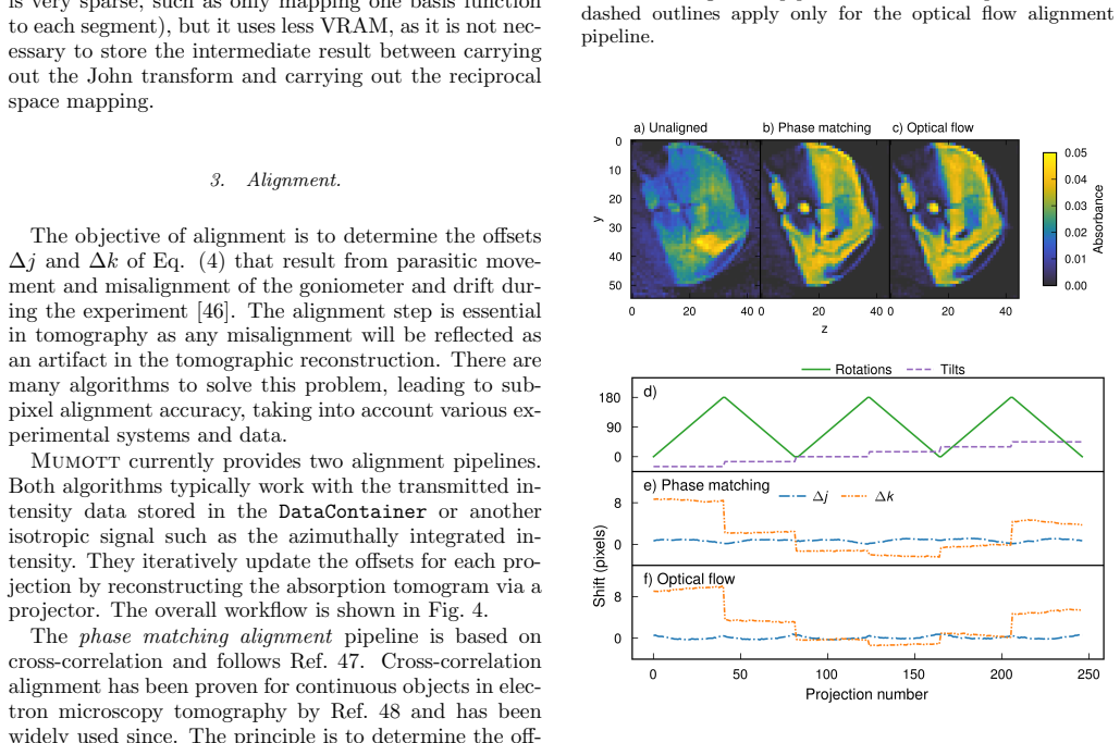
Alignment. The objective of alignment is to determine the offsets ∆j and ∆k of Eq. (4) that result from parasitic move- ment and misalignment of the goniometer and drift dur- ing the experiment [46]. The alignment step is essential in tomography as any misalignment will be ref...
-
[13]
The DataContainer is the owner of the input data, which is stored in HDF5 format
Data and geometry. The DataContainer is the owner of the input data, which is stored in HDF5 format. The input (measure- ments and geometry metadata) is stored as a list of projections, indexed by the direction index s as given in Eq. (5), and the measured tensor tomographic d...
-
[14]
The Projector and BasisSet classes contain the methods and properties needed to compute the forward model defined in Eq
Projectors and basis sets. The Projector and BasisSet classes contain the methods and properties needed to compute the forward model defined in Eq. (7) and its adjoint. The Projector objects depends on a Geometry object and employ rou- tines implemented using the numba package...
-
[15]
The ResidualCalculator is a managing object which takes a DataContainer, Projector, and BasisSet, and uses them to compute residuals
Residual calculation. The ResidualCalculator is a managing object which takes a DataContainer, Projector, and BasisSet, and uses them to compute residuals. It tracks the current reconstruction, i.e., cxyzi. In other words, for the data 10 Dsjkc, and the current reconstruction ...
-
[16]
The goal of the optimization is to minimize a LossFunction (also known as an objective function) by tuning the coefficients of the underlying model by using an Optimizer
Optimization. The goal of the optimization is to minimize a LossFunction (also known as an objective function) by tuning the coefficients of the underlying model by using an Optimizer. The LossFunction combines a ResidualCalculator with one or several Regularizer instances and...
2020
-
[17]
Fratzl and R
P. Fratzl and R. Weinkamer, Nature’s hierarchical mate- rials, Progress in Materials Science 52, 1263 (2007)
2007
-
[18]
Reznikov, R
N. Reznikov, R. Shahar, and S. Weiner, Bone hierarchi- cal structure in three dimensions, Acta Biomaterialia 10, 3815 (2014), biomineralization
2014
-
[19]
Schrauwen, R
B. Schrauwen, R. Janssen, L. Govaert, and H. Meijer, In- trinsic deformation behavior of semicrystalline polymers, Macromolecules 37, 6069 (2004)
2004
-
[20]
Stribeck, U
N. Stribeck, U. N¨ ochel, S. S. Funari, and T. Schu- bert, Tensile tests of polypropylene monitored by saxs. comparing the stretch-hold technique to the dynamic technique, Journal of Polymer Science Part B: Polymer Physics 46, 721 (2008)
2008
-
[21]
Y. Tang, Z. Jiang, Y. Men, L. An, H.-F. F. Enderle, D. Lilge, S. V. Roth, R. Gehrke, and J. Rieger, Uniaxial deformation of overstretched polyethylene: In-situ syn- chrotron small angle x-ray scattering study, Polymer 48, 5125–5132 (2007)
2007
-
[22]
Gantenbein, K
S. Gantenbein, K. Masania, W. Woigk, J. P. W. Sesseg, T. A. Tervoort, and A. R. Studart, Three-dimensional printing of hierarchical liquid-crystal-polymer structures, Nature 561, 226 (2018)
2018
-
[23]
M. Endrizzi, X-ray phase-contrast imaging, Nuclear In- struments and Methods in Physics Research Section A: Accelerators, Spectrometers, Detectors and Associated Equipment 878, 88 (2018)
2018
-
[24]
X. Ou, X. Chen, X. Xu, L. Xie, X. Chen, Z. Hong, H. Bai, X. Liu, Q. Chen, L. Li, and H. Yang, Recent development in x-ray imaging technology: Future and challenges, Re- search 2021 (2021)
2021
-
[25]
Georgiadis, R
M. Georgiadis, R. M¨ uller, and P. Schneider, Techniques to assess bone ultrastructure organization: orientation and arrangement of mineralized collagen fibrils, Journal of The Royal Society Interface 13, 20160088 (2016)
2016
-
[26]
T. H. Jensen, M. Bech, O. Bunk, T. Donath, C. David, R. Feidenhans’l, and F. Pfeiffer, Directional x-ray dark- field imaging, Physics in Medicine & Biology 55, 3317 (2010)
2010
-
[27]
M. Busi, J. Shen, M. Bacak, M. C. Zdora, J. ˇCapek, J. Valsecchi, and M. Strobl, Multi-directional neutron dark-field imaging with single absorption grating, Scien- tific Reports 10.1038/s41598-023-42310-y (2023)
2023 doi
-
[28]
Stribeck, A
N. Stribeck, A. A. Camarillo, U. N¨ ochel, C. Schroer, M. Kuhlmann, S. V. Roth, R. Gehrke, and R. K. Bayer, Volume-resolved nanostructure survey of a poly- mer part by means of saxs microtomography, Macro- molecular Chemistry and Physics 207, 1139 (2006)
2006
-
[29]
C. G. Schroer, M. Kuhlmann, S. V. Roth, R. Gehrke, N. Stribeck, A. Almendarez-Camarillo, and B. Lengeler, Mapping the local nanostructure inside a specimen by to- mographic small-angle x-ray scattering, Applied Physics Letters 88, 164102 (2006)
2006
-
[30]
Kleuker, P
U. Kleuker, P. Suortti, W. Weyrich, and P. Spanne, Fea- sibility study of x-ray diffraction computed tomography for medical imaging, Physics in Medicine & Biology 43, 2911 (1998)
1998
-
[31]
S. R. Stock, F. D. Carlo, and J. D. Almer, High energy x-ray scattering tomography applied to bone, Journal of Structural Biology 161, 144 (2008)
2008
-
[32]
Bleuet, E
P. Bleuet, E. Welcomme, E. Dooryhee, J. Susini, J.-L. Hodeau, and P. Walter, Probing the structure of het- erogeneous diluted materials by diffraction tomography., Nature Materials 7 6, 468 (2008)
2008
-
[33]
Malecki, E
A. Malecki, E. Eggl, F. Schaff, G. Potdevin, T. Baum, E. G. Garcia, J. S. Bauer, and F. Pfeiffer, Correlation of x-ray dark-field radiography to mechanical sample properties, Microscopy and Microanalysis 20, 1528–1533 (2014)
2014
-
[34]
J. Kim, M. Kagias, F. Marone, and M. Stampanoni, X- ray scattering tensor tomography with circular gratings, Applied Physics Letters 116, 134102 (2020)
2020
-
[35]
Liebi, M
M. Liebi, M. Georgiadis, A. Menzel, P. Schneider, J. Kohlbrecher, O. Bunk, and M. Guizar-Sicairos, Nanos- tructure surveys of macroscopic specimens by small-angle scattering tensor tomography, Nature 527, 349 (2015)
2015
-
[36]
Schaff, M
F. Schaff, M. Bech, P. Zaslansky, C. Jud, M. Liebi, M. Guizar-Sicairos, and F. Pfeiffer, Six-dimensional real and reciprocal space small-angle x-ray scattering tomog- raphy, Nature 527, 353 (2015)
2015
-
[37]
Liebi, M
M. Liebi, M. Georgiadis, J. Kohlbrecher, M. Holler, J. Raabe, I. Usov, A. Menzel, P. Schneider, O. Bunk, and M. Guizar-Sicairos, Small-angle X-ray scattering tensor tomography: model of the three-dimensional reciprocal- space map, reconstruction algorithm and angular sam- plin...
2018
-
[38]
Z. Gao, M. Guizar-Sicairos, V. Lutz-Bueno, A. Schr¨ oter, M. Liebi, M. Rudin, and M. Georgiadis, High-speed ten- sor tomography: iterative reconstruction tensor tomog- raphy (IRTT) algorithm, Acta Crystallographica Section A 75, 223 (2019)
2019
-
[39]
L. C. Nielsen, P. Erhart, M. Guizar-Sicairos, and M. Liebi, Small-angle scattering tensor tomography al- gorithm for robust reconstruction of complex textures, Acta Crystallographica Section A 79, 515 (2023)
2023
-
[40]
T. A. Gr¨ unewald, M. Liebi, N. K. Wittig, A. Jo- hannes, T. Sikjaer, L. Rejnmark, Z. Gao, M. Rosenthal, M. Guizar-Sicairos, H. Birkedal, and M. Burghammer, Mapping the 3d orientation of nanocrystals and nanos- tructures in human bone: Indications of novel structural features,...
2020
-
[41]
Donnelly, M
C. Donnelly, M. Guizar-Sicairos, V. Scagnoli, S. Gliga, M. Holler, J. Raabe, and L. J. Heyderman, Three- dimensional magnetization structures revealed with x-ray vector nanotomography, Nature 10.1038/nature23006 (2017)
2017 doi
-
[42]
Sales, M
M. Sales, M. Strobl, T. Shinohara, A. S. Tremsin, L. T. Kuhn, W. R. B. Lionheart, N. M. Desai, A. B. Dahl, and S. Schmidt, Three dimensional polarimetric neutron to- mography of magnetic fields, Scientific Reports 8 (2017)
2017
-
[43]
Kieffer, V
J. Kieffer, V. Valls, N. Blanc, and C. Hennig, New tools for calibrating diffraction setups, Journal of Synchrotron Radiation 27, 558 (2020)
2020
-
[44]
A. B. Jensen, T. E. K. Christensen, C. Weninger, and H. Birkedal, Very large-scale diffraction investigations en- abled by a matrix-multiplication facilitated radial and azimuthal integration algorithm: MatFRAIA, Journal of Synchrotron Radiation 29, 1420 (2022)
2022
-
[45]
B. R. Pauw, Everything saxs: small-angle scattering pat- tern collection and correction, Journal of Physics: Con- densed Matter 25, 383201 (2013)
2013
-
[46]
T. A. Gr¨ unewald, A. Johannes, N. K. Wittig, J. Palle, 13 A. Rack, M. Burghammer, and H. Birkedal, Bone mineral properties and 3D orientation of human lamellar bone around cement lines and the Haversian system, IUCrJ 10, 189 (2023)
2023
-
[47]
M. D. de Jonge and S. Vogt, Hard x-ray fluorescence to- mography—an emerging tool for structural visualization, Current Opinion in Structural Biology 20, 606 (2010)
2010
-
[48]
P. M. Shikhaliev, Energy-resolved computed tomogra- phy: first experimental results, Physics in Medicine & Biology 53, 5595 (2008)
2008
-
[49]
Z. Gao, M. Odstrcil, S. B¨ ocklein, D. Palagin, M. Holler, D. F. Sanchez, F. Krumeich, A. Menzel, M. Stampanoni, G. Mestl, J. A. van Bokhoven, M. Guizar-Sicairos, and J. Ihli, Sparse ab initio x-ray transmission spectrotomog- raphy for nanoscopic compositional analysis of func...
2021
-
[50]
S. K. Lam, A. Pitrou, and S. Seibert, Numba: A llvm- based python jit compiler, in Proceedings of the Second Workshop on the LLVM Compiler Infrastructure in HPC (2015) pp. 1–6
2015
-
[51]
C. R. Harris, K. J. Millman, S. J. van der Walt, R. Gom- mers, P. Virtanen, D. Cournapeau, E. Wieser, J. Tay- lor, S. Berg, N. J. Smith, R. Kern, M. Picus, S. Hoyer, M. H. van Kerkwijk, M. Brett, A. Haldane, J. F. del R´ ıo, M. Wiebe, P. Peterson, P. G´ erard-Marchant, K. Shep...
2020
-
[52]
Virtanen, R
P. Virtanen, R. Gommers, T. E. Oliphant, M. Haber- land, T. Reddy, D. Cournapeau, E. Burovski, P. Pe- terson, W. Weckesser, J. Bright, S. J. van der Walt, M. Brett, J. Wilson, K. J. Millman, N. Mayorov, A. R. J. Nelson, E. Jones, R. Kern, E. Larson, C. J. Carey, ˙I. Po- lat, Y...
2020
-
[53]
Van der Walt, J
S. Van der Walt, J. L. Sch¨ onberger, J. Nunez-Iglesias, F. Boulogne, J. D. Warner, N. Yager, E. Gouillart, and T. Yu, scikit-image: image processing in python, PeerJ 2, e453 (2014)
2014
-
[54]
Kovesi, Good colour maps: How to design them, arXiv (2015), 1509.03700
P. Kovesi, Good colour maps: How to design them, arXiv (2015), 1509.03700
2015 arXiv
-
[55]
Odstrˇ cil, M
M. Odstrˇ cil, M. Holler, J. Raabe, and M. Guizar-Sicairos, Alignment methods for nanotomography with deep sub- pixel accuracy, Optics Express 27, 36637 (2019)
2019
-
[56]
P. J. Basser and C. Pierpaoli, Microstructural and phys- iological features of tissues elucidated by quantitative- diffusion-tensor mri, Journal of Magnetic Resonance, Se- ries B 111, 209 (1996)
1996
-
[57]
L. C. Nielsen, T. T¨ anzer, I. Rodriguez-Fernandez, P. Er- hart, and M. Liebi, Investigating the missing-wedge prob- lem in small-angle X-ray scattering tensor tomography across real and reciprocal space, Journal of Synchrotron Radiation 31, 1327 (2024)
2024
-
[58]
H. J. Bunge, Mathematische Methoden der Texturanalyse (De Gruyter, 1969)
1969
-
[59]
Carlsen, C
M. Carlsen, C. Appel, W. Hearn, M. Olsson, A. Men- zel, and M. Liebi, X-ray tensor tomography for small- grained polycrystals with strong texture, Journal of Ap- plied Crystallography 57 (2024)
2024
-
[60]
Elfving, P
T. Elfving, P. C. Hansen, and T. Nikazad, Semiconver- gence and relaxation parameters for projected sirt algo- rithms, SIAM Journal on Scientific Computing34, A2000 (2012)
2012
-
[61]
Gregor and J
J. Gregor and J. A. Fessler, Comparison of sirt and sqs for regularized weighted least squares image reconstruc- tion, IEEE Transactions on Computational Imaging 1, 44 (2015)
2015
-
[62]
Frank, P
J. Frank, P. Penczek, and W. Liu, Alignment, classifica- tion, and three-dimensional reconstruction of single par- ticles embedded in ice, Scanning Microscopy Supplement 6, 11 (1992)
1992
-
[63]
Guizar-Sicairos, S
M. Guizar-Sicairos, S. T. Thurman, and J. R. Fienup, Efficient subpixel image registration algorithms, Optics Letters 33, 156 (2008)
2008
-
[64]
Guckenberger, Determination of a common origin in the micrographs of tilt series in three-dimensional elec- tron microscopy, Ultramicroscopy 9, 167 (1982)
R. Guckenberger, Determination of a common origin in the micrographs of tilt series in three-dimensional elec- tron microscopy, Ultramicroscopy 9, 167 (1982)
1982
-
[65]
Nielsen, M
L. Nielsen, M. Liebi, M. Guizar-Sicairos, and M. Geor- giadis, Trabecular bone datasets for SAXS Tensor To- mography (2023), doi:10.5281/zenodo.10074598
2023 doi
-
[66]
P. M. Joseph, An improved algorithm for reprojecting rays through pixel images, IEEE Transactions on Medical Imaging 1, 192 (1982)
1982
-
[67]
W. Xu, F. Xu, M. Jones, B. Keszthelyi, J. Sedat, D. Agard, and K. Mueller, High-performance itera- tive electron tomography reconstruction with long-object compensation using graphics processing units (gpus), Journal of Structural Biology 171, 142 (2010)
2010
-
[68]
Palenstijn, K
W. Palenstijn, K. Batenburg, and J. Sijbers, Performance improvements for iterative electron tomography recon- struction using graphics processing units (gpus), Journal of Structural Biology 176, 250 (2011)
2011
-
[69]
P. J. Huber, Robust Estimation of a Location Parameter, The Annals of Mathematical Statistics 35, 73 (1964)
1964
-
[70]
M. P. K. Frewein, J. Mason, B. Maier, H. C¨ olfen, A. Med- jahed, M. Burghammer, M. Allain, and T. A. Gr¨ unewald, Texture tomography, a versatile framework to study crys- talline texture in 3D, IUCrJ 11 (2024)
2024
Reviewed August 16, 2026 · model on record in the stance chip above.
Discussion (0). Continue with ORCID to comment.