REVIEW 2 major objections 4 minor 1 cited by
The Evolution of Earth's Magnetosphere During the Solar Main Sequence
T0 review · 2 major / 4 minor · reviewed 2026-08-14 · deepseek-v4-flash
Pith's one-line read As the Sun spun down, Earth's magnetopause standoff distance grew from about 2.3 Earth radii in a fast-rotating young Sun to 9.4 Earth radii today, following a broken power law in rotation rate; at the most extreme early rotation, no bow…
desk verdict Solid, honest MHD mapping of Earth's magnetospheric evolution, but the no-shock early Sun claim is a knife-edge extrapolation that should be softened. read the letter →
The pith
A machine-rendered reading of the paper's core claim, the machinery that carries it, and where it could break.
The reading
What carries the argument
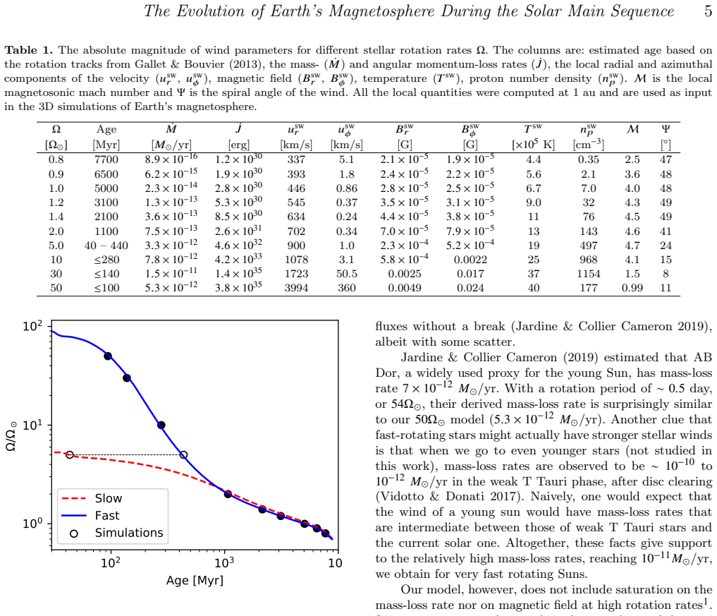
The load-bearing object is the magnetopause standoff distance $r_M$, located in the simulations by the balance of magnetic and thermal pressure on the subsolar line, together with the wind's magnetosonic Mach number $M = u_{sw}^r/\sqrt{v_A^2+c_s^2}$, which sets whether a bow shock exists. The argument is carried by a coupled simulation chain: 1.5D polytropic Weber-Davis wind models use empirical scalings for base temperature (a broken power law breaking at $1.4\,\Omega_{\odot}$), density, and magnetic field with rotation, and the resulting wind properties at 1 au are injected into a 3D ideal MHD magnetosphere model with fixed present-day Earth parameters. The piecewise $r_M(\Omega)$ law is therefore not a magnetospheric effect but a direct consequence of the temperature-rotation scaling; the no-shock result at $50\,\Omega_{\odot}$ depends on the adopted magnetic field-rotation relation staying unsaturated at high rotation.
What would settle it
Concrete test: measure coronal temperatures, wind speeds, and magnetic fields of solar-analogue stars across the rotation range $0.8$-$50\,\Omega_{\odot}$. If the temperature-rotation relation has no break near $1.4\,\Omega_{\odot}$, the predicted $\Omega^{-0.27}/\Omega^{-2.04}$ break in Earth's magnetopause would not occur, and if a $50\,\Omega_{\odot}$ analogue is found to drive a supermagnetosonic wind (Mach $>1$) at 1 au, the no-bow-shock scenario is falsified directly.
Extended reading notes
Core claim
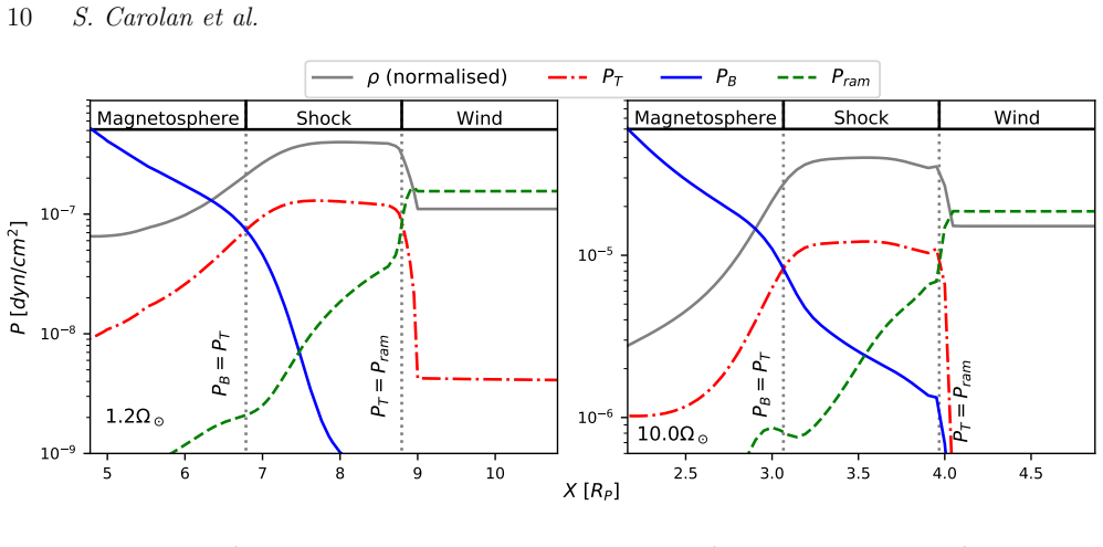
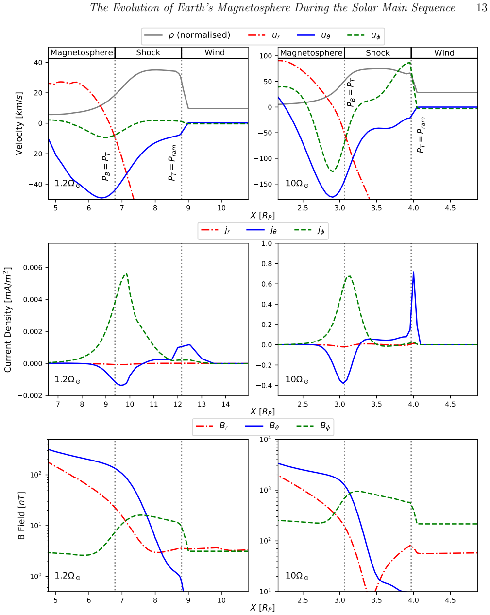
The central discovery is that Earth's magnetosphere, simulated with a constant present-day dipole, responds to the evolving young Sun with a monotonic expansion: $r_M$ grows from about $2.3\,R_p$ at $50\,\Omega_{\odot}$ to $15.9\,R_p$ at $0.8\,\Omega_{\odot}$, with a present-day value of $9.4\,R_p$. The expansion is not a smooth single power law; it follows $r_M \propto \Omega^{-2.04}$ below $1.4\,\Omega_{\odot}$ and $r_M \propto \Omega^{-0.27}$ above it, the break being inherited from a piecewise empirical relation between coronal base temperature and rotation. Along the subsolar line, the bow shock standoff distance is linearly tied to the magnetopause, $r_{BS} = 1.275\,r_M$, for strong-shock models ($\Omega \le 10\,\Omega_{\odot}$), so the magnetosheath thickens in proportion to the magnetosphere. In the speculative fast-rotator scenarios, the wind's magnetosonic Mach number falls to $1.5$ at $30\,\Omega_{\odot}$ and $0.99$ at $50\,\Omega_{\odot}$, producing a weak shock or none at all while the magnetosphere, though compressed to $2.3\,R_p$, still survives.
Load-bearing premise
The load-bearing premise is that the adopted piecewise scaling of coronal base temperature with rotation rate, with its break at $1.4\,\Omega_{\odot}$, is accurate; if it is not, the quoted $\Omega^{-0.27}$ and $\Omega^{-2.04}$ exponents and the position of the break change, and the no-bow-shock result also requires the magnetic-field scaling to remain unsaturated at high rotation.
Editorial extensions
If this is right
- For most of solar main-sequence evolution ($\Omega \le 10\,\Omega_{\odot}$), Earth had a strong bow shock and a magnetosheath thickness proportional to $r_M$, so the whole dayside interaction region scaled with the magnetopause distance.
- If the early Sun was a fast rotator ($10$-$50\,\Omega_{\odot}$), the young Earth's magnetosphere was much smaller (down to $2.3\,R_p$) and the fractional area of open field lines was larger, implying that stellar-wind inflow, rather than plasma collection, dominated atmospheric effects at early ages.
- As the Sun continues to spin down below $1.4\,\Omega_{\odot}$, the steep $\Omega^{-2.04}$ scaling predicts a substantially larger future magnetosphere than today's.
- The absence of a bow shock at $50\,\Omega_{\odot}$ would mean that the young Earth could have been directly exposed to submagnetosonic solar wind plasma, changing the plasma entry routes even though the magnetic shield was not crushed.
Reading between the lines
- If the empirical temperature-rotation break at $1.4\,\Omega_{\odot}$ is real, it should show up as a corresponding break in astrospheric Ly$\alpha$ mass-loss or X-ray temperature surveys of solar analogues; looking for that break would test whether the two-exponent magnetopause law is universal or Sun-specific.
- Because the no-shock prediction rests on the magnetic field-rotation relation remaining unsaturated, a detection of wind saturation in fast rotators (for example, from spin-down torques flattening at high $\Omega$) would remove the bow-shock-free regime without changing the low-rotation results.
- The same simulation chain could be applied to exoplanets: planets around fast-rotating young stars may harbour magnetospheres with no detectable bow shock, which would affect how their winds and magnetic fields are inferred from transit and radio observations.
Signed reviews
Editorial analysis
A structured set of objections, weighed in public.
Referee Report
Summary. This paper couples 1.5D Weber-Davis stellar-wind models, calibrated to empirical rotation-dependent base temperature, density, and magnetic-field relations, with 3D SWMF MHD simulations of Earth's magnetosphere, in order to follow the dayside magnetopause standoff distance and bow shock over the solar main sequence for rotation rates from 0.8 to 50 Omega_sun. The principal results are that the standoff distance is a decreasing broken power law of Omega, with exponent -2.04 below 1.4 Omega_sun and -0.27 above, that the subsolar magnetosheath thickness scales linearly with standoff distance for the strong-shock cases, and that in the extreme assumed 50 Omega_sun wind the flow is submagnetosonic (M=0.99), so no bow shock forms. The paper explicitly attributes the break at 1.4 Omega_sun to the adopted piecewise temperature relation and flags the neglect of wind saturation at high rotation rates.
Significance. If upheld, this is a useful quantitative scenario for the evolution of the paleo-Earth magnetosphere and for how stellar spin-down affects wind-planet coupling more generally. The methods are standard but carefully used: the resolution is tested, the pressure-balance identification of the magnetopause and bow shock is cross-checked against density and velocity profiles and Rankine-Hugoniot jump conditions, and the present-day standoff distance of 9.4 R_p reproduces observed values. The paper is also transparent about age-rotation degeneracies and provides fitting formulas for the wind quantities in Appendix A. The main caveat is that the two headline claims, namely the broken scaling exponents and the absence of a bow shock at 50 Omega_sun, are directly inherited from empirically fitted input scalings and are therefore only as robust as those input relations; the paper does not currently quantify that sensitivity.
major comments (2)
- [Section 4.1, Eqs. (1) and (13)] The conclusion that no bow shock could be present at 50 Omega_sun rests on a magnetosonic Mach number of M=0.99, i.e., within one percent of the shock threshold. This value is produced by the unsaturated wind model, and the paper itself states in Section 2 (footnote 1) and Section 6 that saturation is required to explain the spin-down of fast rotators and that the model over-predicts angular-momentum loss above roughly 10 Omega_sun. Since the magnetic field enters M through v_A and is described by the empirical power law in Eq. (3), a modest change in B within the observational scatter, or a saturated B-Omega relation, can move M above unity and restore a bow shock in the 50 Omega_sun case; the 30 Omega_sun case is similarly marginal. Please provide a sensitivity test of M (and of the resulting magnetospheric state) to the scatter in Eqs. (1)-(3) and to a saturated magnetic-field scaling, or alternatively reformulate the abstract claim as a property of this specific unsaturated model rather than a general prediction.
- [Section 4.1, Eqs. (1) and (13)] The broken power-law exponents for the standoff distance are fits to simulation outputs whose input base temperature T0 is itself a broken power law at 1.4 Omega_sun. The paper is honest that the break is inherited from the empirical temperature relation, but the quantitative exponents -2.04 and -0.27 are still presented without uncertainties. Because these exponents are the central quantitative result, please show how they change when the normalizations and slopes of Eqs. (1)-(3) are varied within their observational scatter, and state which parts of the scaling, if any, are robust. Without such a test, the reader cannot distinguish an empirical interpolation from a physical scaling law.
minor comments (4)
- [Table 1] The values in the Psi column are inconsistent with the definition Psi = arctan(B_phi^sw / B_r^sw) given in Section 2; for example, the 10 Omega_sun row has B_phi^sw / B_r^sw approximately 3.8, corresponding to about 75 degrees, not the tabulated 15 degrees. Either the column lists the complementary angle or the radial and azimuthal columns are mislabeled; please correct this.
- [Section 2.1, Eq. (2)] The units written for n0 are [g/cm3], but the text describes a base number density and the numerical value (10^8 times a dimensionless factor) is in cm^-3. Please correct the unit label.
- [Section 3, Figure 3] The grid is described as a 'cubic grid of length 32 R_p', but the stated range x = [-44, 20] R_p has length 64 R_p. Please reconcile the coordinate range with the stated box size.
- [Section 5, Figure 14] For the 30 and 50 Omega_sun cases, the standoff distance is identified from the j_phi magnetopause current because the pressure-balance method is not usable. Please add some additional validation of this diagnostic, such as a magnetic-field-line connectivity map or a stagnation-point check, since the claim that the magnetosphere is not completely crushed at 50 Omega_sun depends on this identification.
Circularity Check
No significant circularity: the magnetopause scaling and the no-shock case are forward-model outputs from disclosed empirical inputs, not inputs renamed as predictions.
full rationale
This paper is a forward-modeling study: it takes observationally calibrated scalings for stellar wind base temperature, density, and magnetic field (Eqs. 1-3) as inputs to a 1.5D Weber-Davis wind model, then uses the resulting 1-au wind properties as boundary conditions for 3D MHD magnetosphere simulations. The headline piecewise magnetopause scaling (Eq. 13) and the M=0.99 no-shock case at 50 Omega_sun are outputs of those simulations, not parameters fitted to the target quantities. The 1.4 Omega_sun break in r_M is inherited from the adopted piecewise T0(Omega) relation, but the paper states this explicitly: the abstract says "This break is a result of the empirical properties adopted for the solar wind evolution," and Section 4.1 says "This is due to how the base temperature of the winds is specified in Section 2, which is given by a piecewise function about 1.4 Omega_sun." It is therefore a disclosed consequence of an input, not a disguised derivation. The power-law exponents in Eq. 13 are fits to r_M values produced by the coupled simulations, which is standard summarization of model output rather than circular prediction. The self-citations (O'Fionnagain & Vidotto 2018 for T0; Vidotto et al. 2014 for B) are empirical relations based on X-ray observations and magnetic maps, externally falsifiable, and therefore constitute genuine evidence rather than load-bearing self-citation. The acknowledged neglect of wind saturation above roughly 10 Omega_sun (Section 2 and Section 6) makes the 50 Omega_sun no-shock conclusion fragile, but fragility is a robustness and correctness concern, not circularity. No step in the derivation chain is equivalent to its own input by construction.
Assumptions & free parameters
free parameters (6)
- T0 base temperature normalization (Omega < 1.4 Omega_sun) =
1.5e6 K, exponent 1.2
- T0 base temperature normalization (Omega >= 1.4 Omega_sun) =
1.98e6 K, exponent 0.37
- Break rotation Omega_break =
1.4 Omega_sun
- n0 base density normalization =
1e8 (Omega/Omega_sun)^0.6 g/cm3
- B_r,0 base magnetic field normalization =
1.29 (Omega/Omega_sun)^1.32 G
- Polytropic index alpha =
1.05
assumptions (6)
- domain assumption The 1.5D Weber-Davis polytropic wind model with polytropic index alpha = 1.05 and no energy equation adequately describes the solar wind acceleration and magnetic field structure out to 1 au.
- domain assumption The base temperature, density, and radial magnetic field of the wind follow the empirical rotation scalings in Eqs. (1)-(3).
- domain assumption The 1 au wind properties from the 1.5D model can be used as spatially uniform inflow boundary conditions for the 3D magnetosphere simulation.
- domain assumption Earth's dipole moment is constant over the main sequence and the magnetic axis is aligned with the rotation axis.
- ad hoc to paper Stellar wind mass-loss rate and magnetic field do not saturate at high rotation rates.
- standard math The ideal MHD equations with adiabatic index gamma = 5/3 describe the magnetosphere and bow shock.
Cite this review
Pith. "Pith review of The Evolution of Earth's Magnetosphere During the Solar Main Sequence." pith.science (2026). https://pith.science/paper/UP4KJODM
@misc{pith2026190803537,
  author       = {Pith},
  title        = {Pith review of: The Evolution of Earth's Magnetosphere During the Solar Main Sequence},
  year         = {2026},
  howpublished = {\url{https://pith.science/paper/UP4KJODM}},
  note         = {Machine review of arXiv:1908.03537}
}
read the original abstract
As a star spins-down during the main sequence, its wind properties are affected. In this work, we investigate how the Earth's magnetosphere has responded to the change in the solar wind. Earth's magnetosphere is simulated using 3D magnetohydrodynamic models that incorporate the evolving local properties of the solar wind. The solar wind, on the other hand, is modelled in 1.5D for a range of rotation rates Omega from 50 to 0.8 times the present-day solar rotation (Omega_sun). Our solar wind model uses empirical values for magnetic field strengths, base temperature and density, which are derived from observations of solar-like stars. We find that for rotation rates ~10 Omega_sun, Earth's magnetosphere was substantially smaller than it is today, exhibiting a strong bow shock. As the sun spins down, the magnetopause standoff distance varies with Omega^{-0.27} for higher rotation rates (early ages, > 1.4 Omega_sun), and with Omega^{-2.04} for lower rotation rates (older ages, < 1.4 Omega_sun). This break is a result of the empirical properties adopted for the solar wind evolution. We also see a linear relationship between magnetopause distance and the thickness of the shock on the subsolar line for the majority of the evolution (< 10 Omega_sun). It is possible that a young fast rotating Sun would have had rotation rates as high as 30 to 50 Omega_sun. In these speculative scenarios, at 30 Omega_sun, a weak shock would have been formed, but for 50 Omega_sun, we find that no bow shock could be present around Earth's magnetosphere. This implies that with the Sun continuing to spin down, a strong shock would have developed around our planet, and remained for most of the duration of the solar main sequence.
Figures


Figures from the paper (11 more)






Forward citations
Cited by 1 Pith paper
-
A Self-Consistent 3D Hydrodynamic Model for Helium Transit Signatures in Evaporating Hot Jupiters
A 3D hydrodynamic model with self-consistent hydrogen-helium chemistry shows stellar winds compress escaping hot-Jupiter atmospheres and suppress the 1083 nm helium triplet signal, while a young star's strong XUV flux...
Reference graph
Works this paper leans on
-
[1]
Aarnio A. N., Stassun K. G., Hughes W. J., McGregor S. L., 2011, @doi [ ] 10.1007/s11207-010-9672-7 , https://ui.adsabs.harvard.edu/abs/2011SoPh..268..195A 268, 195
-
[2]
Adams F. C., 2011, @doi [ ] 10.1088/0004-637X/730/1/27 , http://adsabs.harvard.edu/abs/2011ApJ...730...27A 730, 27
-
[3]
Airapetian V. S., Glocer A., Gronoff G., H \'e brard E., Danchi W., 2016, @doi [Nature Geoscience] 10.1038/ngeo2719 , http://adsabs.harvard.edu/abs/2016NatGe...9..452A 9, 452
doi:10.1038/ngeo2719 2016
-
[4]
Alvarado-G \'o mez J. D., Drake J. J., Cohen O., Moschou S. P., Garraffo C., 2018, @doi [ ] 10.3847/1538-4357/aacb7f , https://ui.adsabs.harvard.edu/abs/2018ApJ...862...93A 862, 93
-
[5]
Bagenal F., 2013, Planetary Magnetospheres . p. 251, @doi 10.1007/978-94-007-5606-9_6
-
[6]
A., 2013, Physics of Collisionless Shocks: Space Plasma Shock Waves
Balogh A., Treumann R. A., 2013, Physics of Collisionless Shocks: Space Plasma Shock Waves . ISSI Scientific Report Series, Springer, New York, http://cds.cern.ch/record/1517899
-
[7]
A., 2003, @doi [ ] 10.1086/367639 , https://ui.adsabs.harvard.edu/abs/2003ApJ...586..464B 586, 464
Barnes S. A., 2003, @doi [ ] 10.1086/367639 , https://ui.adsabs.harvard.edu/abs/2003ApJ...586..464B 586, 464
doi:10.1086/367639 2003
-
[8]
Beck P. G., et al., 2017, @doi [ ] 10.1051/0004-6361/201629820 , https://ui.adsabs.harvard.edu/abs/2017A&A...602A..63B 602, A63
Show all 75 references
-
[9]
Bharati Das S., Basak A., Nandy D., Vaidya B., 2018, arXiv e-prints, http://adsabs.harvard.edu/abs/2018arXiv181207767B
2018
-
[10]
G., Tarduno J
Blackman E. G., Tarduno J. A., 2018, @doi [ ] 10.1093/mnras/sty2640 , http://adsabs.harvard.edu/abs/2018MNRAS.481.5146B 481, 5146
2018 doi
-
[11]
S., Poppenhaeger K., Watson C
Booth R. S., Poppenhaeger K., Watson C. A., Silva Aguirre V., Wolk S. J., 2017, @doi [ ] 10.1093/mnras/stx1630 , http://adsabs.harvard.edu/abs/2017MNRAS.471.1012B 471, 1012
2017 doi
-
[12]
A., Leblanc F., Luhmann J
Brain D. A., Leblanc F., Luhmann J. G., Moore T. E., Tian F., 2013, Planetary Magnetic Fields and Climate Evolution . pp 487--501, @doi 10.2458/azu_uapress_9780816530595-ch20
2013 doi
-
[13]
Chapman S., Ferraro V. C. A., 1931, @doi [Terrestrial Magnetism and Atmospheric Electricity (Journal of Geophysical Research)] 10.1029/TE036i002p00077 , https://ui.adsabs.harvard.edu/abs/1931TeMAE..36...77C 36, 77
1931 doi
-
[14]
E., 2004, Physics of Solar System Plasmas
Cravens T. E., 2004, Physics of Solar System Plasmas
2004
-
[15]
J., Cohen O., Yashiro S., Gopalswamy N., 2013, @doi [ ] 10.1088/0004-637X/764/2/170 , https://ui.adsabs.harvard.edu/abs/2013ApJ...764..170D 764, 170
Drake J. J., Cohen O., Yashiro S., Gopalswamy N., 2013, @doi [ ] 10.1088/0004-637X/764/2/170 , https://ui.adsabs.harvard.edu/abs/2013ApJ...764..170D 764, 170
2013 doi
-
[16]
Egan H., Jarvinen R., Brain D., 2019, @doi [ ] 10.1093/mnras/stz788 , http://adsabs.harvard.edu/abs/2019MNRAS.486.1283E 486, 1283
2019 doi
-
[17]
Gallet F., Bouvier J., 2013, @doi [ ] 10.1051/0004-6361/201321302 , http://adsabs.harvard.edu/abs/2013A
2013 doi
-
[18]
I., 2004, Physics of the Space Environment
Gombosi T. I., 2004, Physics of the Space Environment
2004
-
[19]
Holzwarth V., Jardine M., 2007, @doi [ ] 10.1051/0004-6361:20066486 , https://ui.adsabs.harvard.edu/abs/2007A&A...463...11H 463, 11
2007 doi
-
[20]
E., 2003, @doi [ ] 10.1086/379192 , http://adsabs.harvard.edu/abs/2003ApJ...599..516I 599, 516
Ivanova N., Taam R. E., 2003, @doi [ ] 10.1086/379192 , http://adsabs.harvard.edu/abs/2003ApJ...599..516I 599, 516
2003 doi
-
[21]
Jardine M., Collier Cameron A., 2019, @doi [ ] 10.1093/mnras/sty2872 , https://ui.adsabs.harvard.edu/abs/2019MNRAS.482.2853J 482, 2853
2019 doi
-
[22]
G., 2016, @doi [Journal of Geophysical Research (Space Physics)] 10.1002/2015JA021950 , http://adsabs.harvard.edu/abs/2016JGRA..121.1413J 121, 1413
Jia X., Kivelson M. G., 2016, @doi [Journal of Geophysical Research (Space Physics)] 10.1002/2015JA021950 , http://adsabs.harvard.edu/abs/2016JGRA..121.1413J 121, 1413
2016 doi
-
[23]
A., Gombosi T
Jia X., Slavin J. A., Gombosi T. I., Daldorff L. K. S., Toth G., Holst B., 2015, @doi [Journal of Geophysical Research (Space Physics)] 10.1002/2015JA021143 , https://ui.adsabs.harvard.edu/abs/2015JGRA..120.4763J 120, 4763
2015 doi
-
[24]
P., G \"u del M., 2015, @doi [ ] 10.1051/0004-6361/201425283 , http://adsabs.harvard.edu/abs/2015A
Johnstone C. P., G \"u del M., 2015, @doi [ ] 10.1051/0004-6361/201425283 , http://adsabs.harvard.edu/abs/2015A
2015 doi
-
[25]
u del M., L \
Johnstone C. P., G \"u del M., L \"u ftinger T., Toth G., Brott I., 2015a, @doi [ ] 10.1051/0004-6361/201425300 , http://adsabs.harvard.edu/abs/2015A
-
[26]
u del M., Brott I., L \
Johnstone C. P., G \"u del M., Brott I., L \"u ftinger T., 2015b, @doi [ ] 10.1051/0004-6361/201425301 , https://ui.adsabs.harvard.edu/abs/2015A&A...577A..28J 577, A28
-
[27]
u ftinger T., Kislyakova K. G., Lammer H., G \
Johnstone C. P., Khodachenko M. L., L \"u ftinger T., Kislyakova K. G., Lammer H., G \"u del M., 2019, @doi [ ] 10.1051/0004-6361/201935279 , https://ui.adsabs.harvard.edu/abs/2019A&A...624L..10J 624, L10
2019 doi
-
[28]
P., 1999, , https://ui.adsabs.harvard.edu/abs/1999A&A...343..251K 343, 251
Keppens R., Goedbloed J. P., 1999, , https://ui.adsabs.harvard.edu/abs/1999A&A...343..251K 343, 251
1999
-
[29]
L., Shaikhislamov I
Khodachenko M. L., Shaikhislamov I. F., Lammer H., Prokopov P. A., 2015, @doi [ ] 10.1088/0004-637X/813/1/50 , http://adsabs.harvard.edu/abs/2015ApJ...813...50K 813, 50
2015 doi
-
[30]
N., Lammer H., Lichtenegger H
Kulikov Y. N., Lammer H., Lichtenegger H. I. M., Penz T., Breuer D., Spohn T., Lundin R., Biernat H. K., 2007, @doi [ ] 10.1007/s11214-007-9192-4 , https://ui.adsabs.harvard.edu/abs/2007SSRv..129..207K 129, 207
2007 doi
-
[31]
Lammer H., et al., 2011, @doi [Origins of Life and Evolution of the Biosphere] 10.1007/s11084-012-9264-7 , https://ui.adsabs.harvard.edu/abs/2011OLEB...41..503L 41, 503
2011 doi
-
[32]
Lammer H., et al., 2012, @doi [Earth, Planets, and Space] 10.5047/eps.2011.04.002 , https://ui.adsabs.harvard.edu/abs/2012EP&S...64..179L 64, 179
2012 doi
-
[33]
T., Nagy A
Ma Y., Russell C. T., Nagy A. F., Toth G., Dong C., Bougher S. W., 2013, AGU Fall Meeting Abstracts, http://adsabs.harvard.edu/abs/2013AGUFM.P13C..05M pp P13C--05
2013
-
[34]
J., et al., 2015, @doi [ ] 10.1002/2015GL065218 , https://ui.adsabs.harvard.edu/abs/2015GeoRL..42.9113M 42, 9113
Ma Y. J., et al., 2015, @doi [ ] 10.1002/2015GL065218 , https://ui.adsabs.harvard.edu/abs/2015GeoRL..42.9113M 42, 9113
2015 doi
-
[35]
P., MacGregor K
Matt S. P., MacGregor K. B., Pinsonneault M. H., Greene T. P., 2012, @doi [ ] 10.1088/2041-8205/754/2/L26 , https://ui.adsabs.harvard.edu/abs/2012ApJ...754L..26M 754, L26
2012 doi
-
[36]
P., Brun A
Matt S. P., Brun A. S., Baraffe I., Bouvier J., Chabrier G., 2015, @doi [ ] 10.1088/2041-8205/799/2/L23 , https://ui.adsabs.harvard.edu/abs/2015ApJ...799L..23M 799, L23
2015 doi
-
[37]
E., Horwitz J
Moore T. E., Horwitz J. L., 2007, @doi [Reviews of Geophysics] 10.1029/2005RG000194 , https://ui.adsabs.harvard.edu/abs/2007RvGeo..45.3002M 45, RG3002
2007 doi
-
[38]
M., Pulkkinen A
Ngwira C. M., Pulkkinen A. A., 2014, AGU Fall Meeting Abstracts, http://adsabs.harvard.edu/abs/2014AGUFMSM31A4166N pp SM31A--4166
2014
-
[39]
\'O Fionnag \'a in D., et al., 2019, @doi [ ] 10.1093/mnras/sty3132 , https://ui.adsabs.harvard.edu/abs/2019MNRAS.483..873O 483, 873
2019 doi
-
[40]
A., 2018, @doi [ ] 10.1093/mnras/sty394 , http://adsabs.harvard.edu/abs/2018MNRAS.476.2465O 476, 2465
O'Fionnag \'a in D., Vidotto A. A., 2018, @doi [ ] 10.1093/mnras/sty394 , http://adsabs.harvard.edu/abs/2018MNRAS.476.2465O 476, 2465
2018 doi
-
[41]
E., Adams F
Owen J. E., Adams F. C., 2014, @doi [ ] 10.1093/mnras/stu1684 , http://adsabs.harvard.edu/abs/2014MNRAS.444.3761O 444, 3761
2014 doi
-
[42]
Pizzolato N., Maggio A., Micela G., Sciortino S., Ventura P., 2003, @doi [ ] 10.1051/0004-6361:20021560 , https://ui.adsabs.harvard.edu/abs/2003A
2003 doi
-
[43]
W., Kopp R
Pneuman G. W., Kopp R. A., 1971, @doi [ ] 10.1007/BF00145940 , https://ui.adsabs.harvard.edu/abs/1971SoPh...18..258P 18, 258
1971 doi
-
[44]
J., 2018, @doi [ ] 10.3847/1538-4357/aaaebb , http://adsabs.harvard.edu/abs/2018ApJ...856...53P 856, 53
Pognan Q., Garraffo C., Cohen O., Drake J. J., 2018, @doi [ ] 10.3847/1538-4357/aaaebb , http://adsabs.harvard.edu/abs/2018ApJ...856...53P 856, 53
2018 doi
-
[45]
P., Strugarek A., Brun A
R \'e ville V., Folsom C. P., Strugarek A., Brun A. S., 2016, @doi [ ] 10.3847/0004-637X/832/2/145 , https://ui.adsabs.harvard.edu/abs/2016ApJ...832..145R 832, 145
2016 doi
-
[46]
F., G \"u del M., Audard M., 2005, @doi [ ] 10.1086/427977 , http://adsabs.harvard.edu/abs/2005ApJ...622..680R 622, 680
Ribas I., Guinan E. F., G \"u del M., Audard M., 2005, @doi [ ] 10.1086/427977 , http://adsabs.harvard.edu/abs/2005ApJ...622..680R 622, 680
2005 doi
-
[47]
J., De Zeeuw D
Ridley A. J., De Zeeuw D. L., Gombosi T. I., Powell K. G., 2001, @doi [ ] 10.1029/2000JA002233 , https://ui.adsabs.harvard.edu/abs/2001JGR...10630067R 106, 30067
2001 doi
-
[48]
Sakai S., Seki K., Terada N., Shinagawa H., Tanaka T., Ebihara Y., 2018, @doi [ ] 10.1029/2018GL079972 , https://ui.adsabs.harvard.edu/abs/2018GeoRL..45.9336S 45, 9336
2018 doi
-
[49]
M., Airapetian V., Petro N
Saxena P., Killen R. M., Airapetian V., Petro N. E., Curran N. M., Mandell A. M., 2019, @doi [ ] 10.3847/2041-8213/ab18fb , https://ui.adsabs.harvard.edu/abs/2019ApJ...876L..16S 876, L16
2019 doi
-
[50]
A., Petit P., Marsden S
See V., Jardine M., Vidotto A. A., Petit P., Marsden S. C., Jeffers S. V., do Nascimento J. D., 2014, @doi [ ] 10.1051/0004-6361/201424323 , https://ui.adsabs.harvard.edu/abs/2014A&A...570A..99S 570, A99
2014 doi
-
[51]
Skumanich A., 1972, @doi [ ] 10.1086/151310 , http://adsabs.harvard.edu/abs/1972ApJ...171..565S 171, 565
1972 doi
-
[52]
R., Summers A
Spreiter J. R., Summers A. L., Alksne A. Y., 1966, @doi [Planetary and Space Science] https://doi.org/10.1016/0032-0633(66)90124-3 , 14, 223
1966 doi
-
[53]
G., Cohen O., Drake J
Sterenborg M. G., Cohen O., Drake J. J., Gombosi T. I., 2011, @doi [Journal of Geophysical Research (Space Physics)] 10.1029/2010JA016036 , http://adsabs.harvard.edu/abs/2011JGRA..116.1217S 116, A01217
2011 doi
-
[54]
J., Russell C
Strangeway R. J., Russell C. T., Luhmann J. G., Moore T. E., Foster J. C., Barabash S. V., Nilsson H., 2010, AGU Fall Meeting Abstracts, http://adsabs.harvard.edu/abs/2010AGUFMSM33B1893S
2010
-
[55]
A., et al., 2010, @doi [Science] 10.1126/science.1183445 , http://adsabs.harvard.edu/abs/2010Sci...327.1238T 327, 1238
Tarduno J. A., et al., 2010, @doi [Science] 10.1126/science.1183445 , http://adsabs.harvard.edu/abs/2010Sci...327.1238T 327, 1238
2010 doi
-
[56]
A., Blackman E
Tarduno J. A., Blackman E. G., Mamajek E. E., 2014, @doi [Physics of the Earth and Planetary Interiors] 10.1016/j.pepi.2014.05.007 , https://ui.adsabs.harvard.edu/abs/2014PEPI..233...68T 233, 68
2014 doi
-
[57]
N., Lammer H., Lichtenegger H
Terada N., Kulikov Y. N., Lammer H., Lichtenegger H. I. M., Tanaka T., Shinagawa H., Zhang T., 2009a, @doi [Astrobiology] 10.1089/ast.2008.0250 , https://ui.adsabs.harvard.edu/abs/2009AsBio...9...55T 9, 55
2008
-
[58]
Terada N., Shinagawa H., Tanaka T., Murawski K., Terada K., 2009b, @doi [Journal of Geophysical Research (Space Physics)] 10.1029/2008JA013937 , https://ui.adsabs.harvard.edu/abs/2009JGRA..114.9208T 114, A09208
-
[59]
T \'o th G., 1996, Astrophysical Letters and Communications, http://adsabs.harvard.edu/abs/1996ApL
1996
-
[60]
T \'o th G., et al., 2005, @doi [Journal of Geophysical Research (Space Physics)] 10.1029/2005JA011126 , http://adsabs.harvard.edu/abs/2005JGRA..11012226T 110, A12226
2005 doi
-
[61]
B., Arras P., Li Z.-Y., 2011, @doi [ ] 10.1088/0004-637X/728/2/152 , http://adsabs.harvard.edu/abs/2011ApJ...728..152T 728, 152
Trammell G. B., Arras P., Li Z.-Y., 2011, @doi [ ] 10.1088/0004-637X/728/2/152 , http://adsabs.harvard.edu/abs/2011ApJ...728..152T 728, 152
2011 doi
-
[62]
Vidotto A., 2013, @doi [Astronomy and Geophysics] 10.1093/astrogeo/ats038 , https://ui.adsabs.harvard.edu/abs/2013A&G....54a1.25V 54, 1.25
2013 doi
-
[63]
A., 2018, Stellar Coronal and Wind Models: Impact on Exoplanets
Vidotto A. A., 2018, Stellar Coronal and Wind Models: Impact on Exoplanets . p. 26, @doi 10.1007/978-3-319-55333-7_26
2018 doi
-
[64]
A., Donati J
Vidotto A. A., Donati J. F., 2017, @doi [ ] 10.1051/0004-6361/201629700 , https://ui.adsabs.harvard.edu/abs/2017A&A...602A..39V 602, A39
2017 doi
-
[65]
A., Opher M., Jatenco-Pereira V., Gombosi T
Vidotto A. A., Opher M., Jatenco-Pereira V., Gombosi T. I., 2009, @doi [ ] 10.1088/0004-637X/703/2/1734 , http://adsabs.harvard.edu/abs/2009ApJ...703.1734V 703, 1734
2009 doi
-
[66]
A., Jardine M., Morin J., Donati J
Vidotto A. A., Jardine M., Morin J., Donati J. F., Lang P., Russell A. J. B., 2013, @doi [ ] 10.1051/0004-6361/201321504 , https://ui.adsabs.harvard.edu/abs/2013A&A...557A..67V 557, A67
2013 doi
-
[67]
A., et al., 2014, @doi [ ] 10.1093/mnras/stu728 , http://adsabs.harvard.edu/abs/2014MNRAS.441.2361V 441, 2361
Vidotto A. A., et al., 2014, @doi [ ] 10.1093/mnras/stu728 , http://adsabs.harvard.edu/abs/2014MNRAS.441.2361V 441, 2361
2014 doi
-
[68]
A., et al., 2016, @doi [ ] 10.1093/mnrasl/slv147 , https://ui.adsabs.harvard.edu/abs/2016MNRAS.455L..52V 455, L52
Vidotto A. A., et al., 2016, @doi [ ] 10.1093/mnrasl/slv147 , https://ui.adsabs.harvard.edu/abs/2016MNRAS.455L..52V 455, L52
2016 doi
-
[69]
H., Gombosi T
Vogt J., Zieger B., Stadelmann A., Glassmeier K. H., Gombosi T. I., Hansen K. C., Ridley A. J., 2004, @doi [Journal of Geophysical Research (Space Physics)] 10.1029/2003JA010273 , https://ui.adsabs.harvard.edu/abs/2004JGRA..10912221V 109, A12221
2004 doi
-
[70]
J., Davis Jr
Weber E. J., Davis Jr. L., 1967, @doi [ ] 10.1086/149138 , http://adsabs.harvard.edu/abs/1967ApJ...148..217W 148, 217
1967 doi
-
[71]
E., M \"u ller H.-R., Zank G
Wood B. E., M \"u ller H.-R., Zank G. P., Linsky J. L., 2002, @doi [ ] 10.1086/340797 , https://ui.adsabs.harvard.edu/abs/2002ApJ...574..412W 574, 412
2002 doi
-
[72]
E., M \"u ller H
Wood B. E., M \"u ller H. R., Zank G. P., Linsky J. L., Redfield S., 2005, @doi [ ] 10.1086/432716 , https://ui.adsabs.harvard.edu/abs/2005ApJ...628L.143W 628, L143
2005 doi
-
[73]
E., M \"u ller H.-R., Redfield S., Edelman E., 2014, @doi [ ] 10.1088/2041-8205/781/2/L33 , https://ui.adsabs.harvard.edu/abs/2014ApJ...781L..33W 781, L33
Wood B. E., M \"u ller H.-R., Redfield S., Edelman E., 2014, @doi [ ] 10.1088/2041-8205/781/2/L33 , https://ui.adsabs.harvard.edu/abs/2014ApJ...781L..33W 781, L33
2014 doi
-
[75]
I., Bustamante S., Cuartas P
Zuluaga J. I., Bustamante S., Cuartas P. A., Hoyos J. H., 2013b, @doi [ ] 10.1088/0004-637X/770/1/23 , https://ui.adsabs.harvard.edu/abs/2013ApJ...770...23Z 770, 23
-
[76]
L., Ceillier T., Metcalfe T
van Saders J. L., Ceillier T., Metcalfe T. S., Silva Aguirre V., Pinsonneault M. H., Garc \' a R. A., Mathur S., Davies G. R., 2016, @doi [ ] 10.1038/nature16168 , http://adsabs.harvard.edu/abs/2016Natur.529..181V 529, 181
2016 doi
Reviewed August 14, 2026 · model on record in the stance chip above.
Discussion (0). Continue with ORCID to comment.