REVIEW 3 major objections 4 minor 13 cited by
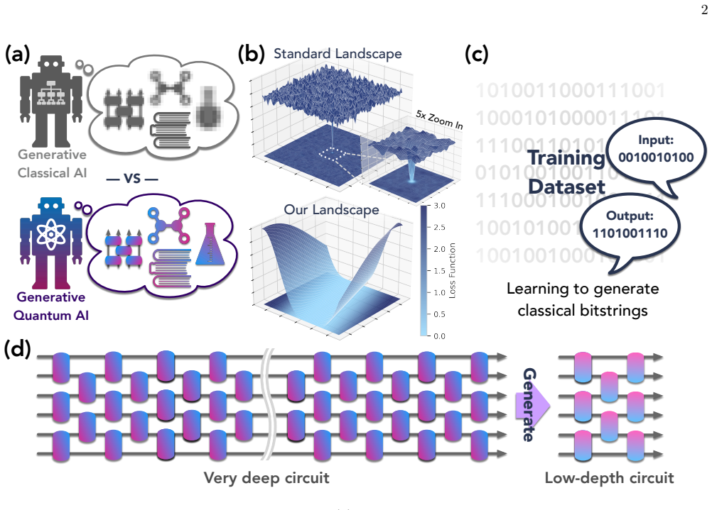
This paper claims generative quantum advantage: families of shallow quantum circuits, called instantaneously-deep QNNs, are both efficiently trainable from classical data and classically hard to sample, with experimental support on a 68-qub
Reviewed by Pith at T0; open to challenge. T0 means a machine referee read the full paper against a public rubric. the ladder, T0–T4 →
T0 review · deepseek-v4-flash
2026-08-04 19:47 UTC pith:VFR6WSAD
load-bearing objection Strong theory, solid small-scale experiment, but the headline beyond-classical claim is inferred, not measured, and the abstract overstates it. the 3 major comments →
Generative quantum advantage for classical and quantum problems
The pith
A machine-rendered reading of the paper's core claim, the machinery that carries it, and where it could break.
Core claim
The central discovery is a family of generative quantum models — instantaneously-deep QNNs — that are universal for classical conditional distributions, efficiently trainable from classical examples, and classically hard to sample from under standard complexity assumptions. The paper proves (Theorem 13) that learning these models is quantumly easy but classically hard: a classical computer can find the parameters from data, but generating new samples requires a quantum computer. The same machinery yields a second result (Theorem 14): finding a constant-depth representation of a circuit promised to have one is classically hard unless BPP=BQP, so circuit compression for fast-forwardable simula
What carries the argument
The key mechanism is the instantaneously-deep QNN: a constant-depth circuit of Hadamard and CZ gates on a D-dimensional lattice whose output distribution exactly equals that of a depth-n deep circuit on a (D-1)-dimensional lattice, via quantum teleportation (measurement-based quantum computation). This exact deep-to-shallow mapping lets a 68-qubit processor sample from distributions that look like much larger shallow circuits. The other load-bearing tool is the sewing technique, which uses ancilla qubits to coherently combine learned local inversions of a shallow unitary into a global constant-depth circuit, provably rendering optimization landscapes benign (strongly convex or with a constan
Load-bearing premise
The load-bearing premise is that the trained shallow model, once learned by emulation, performs on real hardware as well as the original random circuit sampling data, because the exact mapping transfers the XEB fidelity; this transfer from emulation to hardware is not directly measured at the largest sizes.
What would settle it
Run the trained IDQNN at 816 shallow qubits (68 physical qubits) on hardware with no error mitigation and compare the measured XEB on input x=0^n with the XEB of the corresponding deep random circuit sampling data; if the trained circuit's XEB falls substantially below the proxy value, the claim of experimental beyond-classical performance would be falsified.
If this is right
- If the central claim holds, there exist distributions that are both efficiently learnable and beyond-classical to sample, so generative quantum advantage is achievable with near-term hardware.
- The sewing technique implies that shallow quantum circuits can be learned in polynomial time from polynomial data with no barren plateaus, making a broad class of quantum models trainable.
- The hardness of circuit compression means no efficient classical compiler can generally find constant-depth representations even when promised one, so quantum hardware is necessary for this generative task.
- The experiments indicate that with about 10^6 samples an IDQNN can be learned to gate-precision below NISQ error, and inference can outperform classical simulation by a large margin, quantifying practical resource crossovers.
- Both learning and sampling can be performed efficiently in the beyond-classical regime, completing the loop from random circuit sampling to a full generative quantum advantage.
Where Pith is reading between the lines
- The exact deep-to-shallow mapping transfers hardness in both directions: if IDQNN sampling were classically simulable, so would be deep random circuit sampling; conversely, any improvement in deep-circuit sampling algorithms immediately weakens the generative advantage.
- The resource estimate of 34,304 shallow qubits is an upper bound from one particular mapping; more efficient deep-to-shallow mappings could lower the bar for beyond-classical generative learning.
- The sewing-based divide-and-conquer may generalize to learning other structured unitaries beyond constant depth, such as circuits with logarithmic depth or commuting gates, yielding a broader class of trainable quantum models.
- The classical-hardness result for circuit compression could inform verifiable quantum advantage protocols, since it shows that even with a promise, finding a shallow representation is an inherently quantum task.
Editorial analysis
A structured set of objections, weighed in public.
Referee Report
Summary. The paper introduces instantaneously-deep quantum neural networks (IDQNNs), a family of shallow quantum generative models that are claimed to be efficiently trainable from classical data and classically hard to sample from under the assumption that the non-uniform polynomial hierarchy does not collapse (Theorems 12-13). It also proves that finding constant-depth circuit representations promised to exist is classically hard unless BPP=BQP (Theorem 14), and that a divide-and-conquer 'sewing' technique yields benign optimization landscapes (Theorems 4-5). Experimentally, the authors train IDQNNs on a 68-qubit superconducting processor to learn bitstring distributions and to compress a hidden-structure Hamiltonian evolution, reporting a scaling advantage over classical ML baselines. A further result infers beyond-classical performance at 34,304 effective shallow qubits by mapping circuits from Ref. [30] into IDQNN form and borrowing their reported XEB values.
Significance. The theoretical framework is substantial. If it holds, the paper would close an important loop between efficient learning of shallow quantum circuits and known hardness of sampling, with explicit proofs in Appendices F-H, concrete sample-complexity predictions (about 1e6 samples to reach 1e-3 gate fidelity), and a clean formal statement of the hardness assumption. The circuit-compression experiment on 40 qubits and the landscape numerics are also useful and support the trainability claims. The main weakness is experimental: the direct hardware data stop at 816 shallow qubits, a regime the authors themselves classify as classically simulatable, and the beyond-classical number is inferred from a proxy that is not validated against a noise model.
major comments (3)
- [Appendix C.2.c, Fig. 2e] The beyond-classical experimental claim is inferred rather than measured. The manuscript uses the reported XEB values of Ref. [30] as a proxy for the trained IDQNN's hardware performance, justified by an 'exact circuit correspondence.' However, the mapped IDQNN corresponds to 34,304 shallow qubits = 67 x 512 time steps, whereas the Ref. [30] XEB values were obtained at the native depth of those circuits. Transferring XEB requires the mapped deep circuit to have comparable depth, gate count, and error structure; no noise-model calculation or direct measurement of the mapped circuit is provided. Since XEB decays exponentially with accumulated gate error, the expected hardware XEB of a 512-layer mapped circuit is likely far below the quoted values. The caption claim that 'even with hardware noise, quantum models outperform...' is therefore unsupported.
- [Section III (Experiments on learning to generate bitstrings)] The only direct hardware data are for up to 816 shallow qubits, and the paper itself states that '816 shallow qubits are not yet expected to be in the beyond-classical regime.' Thus there is no direct experimental demonstration of generative quantum advantage in the beyond-classical regime; the abstract's claim that the 68-qubit processor demonstrates capabilities 'in the beyond-classical regime' relies entirely on the surrogate in Fig. 2e. This wording should be corrected, and the surrogate should either be supported by a noise-model calculation or removed.
- [Appendix C.2.c, step 1] The 'exact circuit correspondence' is not demonstrated at the level needed to license the proxy. Mapping arbitrary Ref. [30] random-circuit-sampling circuits into the H/RZ/CZ form of the IDQNN, and through a 1D deep layout, requires refitting and recompilation, which changes the two-qubit gate count, depth, and connectivity. The resulting overhead factor (512 time steps for 67 physical qubits) is quoted without derivation. The paper should provide the explicit compiled circuit, its total gate count and depth, and an estimate of its XEB under the device error rates in Appendix B, or present a direct measurement of the mapped circuit.
minor comments (4)
- [Abstract and Fig. 2e caption] The abstract states the processor demonstrates capabilities 'in the beyond-classical regime,' but the direct experiment reaches only 816 shallow qubits, which the text later admits is not beyond classical. Please rephrase to distinguish measured from inferred results.
- [Appendix C.2.c] The sentence 'specialized to the case of x=000..., y=000...' is immediately followed by 'in the case of an all 1 input state,' which is inconsistent. Please clarify whether the hard inference input is all-zero or all-one.
- [Appendix C.2.c] The formula 'FrontierFLOPS target fidelity = FrontierFLOPS perfect fidelity * F_target' is difficult to read; please format properly and define each quantity.
- [Appendix B / Fig. 2] XEB is used both as a fidelity metric and as a training-performance metric. Please define once in the main text how XEB values are computed for the trained models and how they relate to the hardware error rates reported in Appendix B.
Circularity Check
Fig. 2e 'beyond-classical' XEB is Ref [30]'s XEB reused as the trained IDQNN's performance; the 34,304-shallow-qubit advantage is a relabeled prior result rather than a measurement of the new model.
specific steps
-
renaming known result
[Appendix C.2.c 'Beyond classical performance', Fig. 2e; main text 'Experiments on learning to generate bitstrings']
"As we are able to learn from data efficiently in these circuits to beyond the precision of the machine implementing these experiments in addition to an exact circuit correspondence, we use as a proxy for our performance on these circuits their reported XEB values."
The paper's inferred beyond-classical performance (34,304 shallow qubits) is defined to be the XEB values measured in Ref. [30] on the original RCS circuits. The trained IDQNN is never run on hardware in this regime, and no noise-model calculation for the mapped deep circuit is provided. Thus the headline 'generative quantum advantage' in the beyond-classical regime reduces by construction to the prior RCS XEB result, re-expressed as the learned generative model's performance. The mapping is asserted as exact, but the XEB proxy is an identity substitution, not an independent prediction.
full rationale
Most of the paper is self-contained and not circular. Theorems 12 and 13 are proven in Appendices F and H, including a full proof of the shallow-circuit learning theorem (Theorem 8) and standard complexity reductions (Proposition 4); the citations to Ref. [45] are backed by in-paper proofs. The 816-shallow-qubit hardware experiment is a genuine measurement on 68 physical qubits. However, the paper's marquee beyond-classical experimental evidence (Fig. 2e, 'inferred results beyond 34,000 shallow qubits') is not a measurement of the trained IDQNN: the plotted XEB equals Ref. [30]'s reported XEB, by the paper's own statement. This is a renaming/importation of a prior result rather than a derivation from the new model, and the 'exact circuit correspondence' that would license the proxy is asserted without a hardware check or noise analysis. One significant circular/imported step, partial circularity, warrants a 6 rather than a lower score. The paper's transparency about the proxy is a limitation, but it does not remove the by-construction equivalence.
Axiom & Free-Parameter Ledger
free parameters (2)
- IDQNN parameters beta_j (one per qubit) =
learned from classical samples to precision 1e-3 in experiments
- Input distribution D(x) mixture weights =
1/3 for x=0^n, 1/3 i.i.d. p=0.6, 1/3 i.i.d. p=0.2
axioms (5)
- domain assumption Non-uniform polynomial hierarchy does not collapse (Conjecture 1)
- domain assumption BPP != BQP
- domain assumption Promise that a constant-depth representation exists for the target circuit
- domain assumption Local decoupling property of the input distribution D(x)
- standard math Universality of H, RZ, CZ gate set with polynomial overhead (Fact 1)
Cite this review
Pith. "Pith review of Generative quantum advantage for classical and quantum problems." pith.science (2026). https://pith.science/paper/VFR6WSAD
@misc{pith2026250909033,
  author       = {Pith},
  title        = {Pith review of: Generative quantum advantage for classical and quantum problems},
  year         = {2026},
  howpublished = {\url{https://pith.science/paper/VFR6WSAD}},
  note         = {Machine review of arXiv:2509.09033}
}
read the original abstract
Recent breakthroughs in generative machine learning, powered by massive computational resources, have demonstrated unprecedented human-like capabilities. While beyond-classical quantum experiments can generate samples from classically intractable distributions, their complexity has thwarted all efforts toward efficient learning. This challenge has hindered demonstrations of generative quantum advantage: the ability of quantum computers to learn and generate desired outputs substantially better than classical computers. We resolve this challenge by introducing families of generative quantum models that are hard to simulate classically, are efficiently trainable, exhibit no barren plateaus or proliferating local minima, and can learn to generate distributions beyond the reach of classical computers. Using a $68$-qubit superconducting quantum processor, we demonstrate these capabilities in two scenarios: learning classically intractable probability distributions and learning quantum circuits for accelerated physical simulation. Our results establish that both learning and sampling can be performed efficiently in the beyond-classical regime, opening new possibilities for quantum-enhanced generative models with provable advantage.
Figures


Forward citations
Cited by 13 Pith papers
-
Lie Group Diffusion Models for Hardware-Aware Quantum Circuit Synthesis
Lie group diffusion models combine a discrete circuit skeleton selector with continuous diffusion on SU(2) ≃ S³ to synthesize hardware-aware quantum circuits, outperforming baselines on three-qubit Hamiltonian simulat...
-
Quantum Fourier Generative Models Trainable at Large Scale
Quantum Fourier generative models are trained classically at over 1000-qubit scale using log-likelihood loss from Parseval's identity and deployed on superconducting hardware for fast sampling that preserves multi-mod...
-
Gated QKAN-FWP: Scalable Quantum-inspired Sequence Learning
Gated QKAN-FWP combines fast weight programming with quantum-inspired Kolmogorov-Arnold networks via single-qubit DARUAN activations and gated updates to deliver a 12.5k-parameter model that outperforms larger classic...
-
Adversarial Effects on Expressibility and Trainability in Distributed Variational Quantum Algorithms
Adversaries perturbing shared entanglement in distributed VQAs can manipulate a new Kraus expressibility metric to keep gradients large but steer training to incorrect solutions.
-
Minimizing classical resources in variational measurement-based quantum computation for generative modeling
A VMBQC model restricted to one extra trainable parameter generates distributions that the corresponding unitary model cannot learn.
-
Exponential quantum advantage in processing massive classical data
A polylog-sized quantum computer achieves exponential advantage over classical machines in classification and dimension reduction of massive classical data using quantum oracle sketching combined with classical shadows.
-
Toward Generative Quantum Utility via Correlation-Complexity Map
A pre-training diagnostic map based on spectral correlation resemblance to IQP circuits and excess structural complexity identifies suitable datasets like turbulence data for quantum generative models, yielding compet...
-
Quantum computation at the edge of chaos
Topological entanglement entropy regularizes variational quantum algorithms to enforce quantum sparsity and operate at the edge of chaos for better trainability.
-
Scaling Quantum Machine Learning without Tricks: Full-Resolution and Diverse Image Generation
A single end-to-end quantum generator using an image-tailored circuit and learnable multimodal noise achieves state-of-the-art simulated FID scores on full MNIST and Fashion-MNIST without tricks.
-
Software Between Quantum and Machine Learning -- And Down to Pulses
A JAX-based framework extending quantum machine learning to pulse-level control with composable ansatzes, end-to-end optimization, and Fourier diagnostics.
-
Spectral methods: crucial for machine learning, natural for quantum computers?
Quantum computers may enable more natural manipulation of Fourier spectra in ML models via the Quantum Fourier Transform, potentially leading to resource-efficient spectral methods.
-
Generative IQP Circuit Learning with Physics-Informed Latent Initialization
Initializing the latent block of an IQP generative circuit with a PINN-learned latent vector lowers reconstruction error at unseen viscosities versus random initialization on Burgers' equation.
-
Software Between Quantum and Machine Learning -- And Down to Pulses
Introduces a JAX-based framework for pulse-level QML with composable ansatze, end-to-end pulse optimization, and Fourier-analytic diagnostics.
Reference graph
Works this paper leans on
-
[1]
Sample an input product state|𝜓ℓ⟩= ⨂︀𝑛 𝑖=1|𝜓ℓ,𝑖⟩, with each|𝜓 ℓ,𝑖⟩being a uniformly random single-qubit stabilizer state from{|0⟩,|1⟩,|+⟩,|−⟩,|𝑦+⟩,|𝑦−⟩}
-
[2]
Apply the unknown unitary𝑈to|𝜓 ℓ⟩
-
[3]
The measurement collapses the state to a product state|𝜑ℓ⟩= ⨂︀𝑛 𝑖=1|𝜑ℓ,𝑖⟩
Measure each qubit of𝑈|𝜓ℓ⟩in a random Pauli basis chosen from{𝑋, 𝑌, 𝑍}. The measurement collapses the state to a product state|𝜑ℓ⟩= ⨂︀𝑛 𝑖=1|𝜑ℓ,𝑖⟩. This dataset can be represented efficiently on a classical computer using𝒪(𝑁 𝑛)bits. F.2. Algorithm 1: Known structure with direct Heisenberg sewing We begin by presenting an algorithm for learning a shallow qu...
-
[4]
Use Lemma 1 to learn the Heisenberg-evolved Pauli observables^𝑂𝑖,𝑃≈𝑈†𝑃𝑖𝑈
-
[5]
For each qubit𝑖, optimize a local inversion𝑉𝑖 such that𝑉† 𝑖 ^𝑂𝑖,𝑃 𝑉𝑖≈𝑃 𝑖 as in Algorithm 2
-
[6]
Apply local inversion sewing as in Algorithm 2 to obtain the learned channel^ℰ(𝜌). In the following, we state the main lemma for learning the Heisenberg-evolved observables from the dataset𝒯𝑈(𝑁) with an arbitrary circuit architecture for the unknown shallow quantum neural network. Lemma 1(Learning Heisenberg-evolved Pauli observables).Given an unknown𝑛-qu...
-
[7]
For all𝑄∈ {𝐼, 𝑋, 𝑌, 𝑍}⊗𝑛 with|𝑄| ≤𝑘, i.e.,𝑄acts as non-identity on at most𝑘qubits, compute the coefficient: ^𝛼𝑄 = 3|𝑄| 𝑁 𝑁∑︁ ℓ=1 3⟨𝜑 ℓ,𝑖|𝑃|𝜑 ℓ,𝑖⟩·⟨𝜓 ℓ|𝑄|𝜓 ℓ⟩,(S.4.18) then apply a threshold function to the coefficient: ^𝛽𝑄 = {︃ ^𝛼𝑄,|^𝛼 𝑄|≥0.5𝜀/(2 √ 2)𝑘 0,|^𝛼 𝑄|<0.5𝜀/(2 √ 2)𝑘 .(S.4.19)
-
[8]
barren plateau problem
Construct the approximation as: ^𝑂𝑖,𝑃 = ∑︁ 𝑄:|𝑄|≤𝑘 ^𝛽𝑄𝑄.(S.4.20) This algorithm guarantees that with probability at least1−𝛿: ‖ ^𝑂𝑖,𝑃−𝑈†𝑃𝑖𝑈‖∞≤𝜀andsupp( ^𝑂𝑖,𝑃 )⊆supp(𝑈 †𝑃𝑖𝑈)(S.4.21) for all𝑖∈{1, . . . , 𝑛}and𝑃∈{𝑋, 𝑌, 𝑍}, wheresupp(𝐴)is the set of qubits that𝐴acts nontrivially on. F.5. Main learning theorem Theorem 8(Learning shallow quantum circuits).Given...
-
[9]
Every local minimum is global
-
[10]
Proof.These properties follow directly from strong convexity: strictly convex functions have a unique global mini- mizer, and any stationary point must be this minimum
Every critical point satisfies⃗ 𝛼=⃗ 𝛼*. Proof.These properties follow directly from strong convexity: strictly convex functions have a unique global mini- mizer, and any stationary point must be this minimum. G.2.b. Constant local minima in learning local inversions We now analyze the landscape for the non-convex optimization problem underlying Algorithms...
-
[11]
Encodes the input bitstring𝑥∈{0,1} 𝑛 into anℓ-qubit input product state|𝜓 𝑥⟩and a local measurement basisℳ 𝑥 over𝑚≤ℓqubits
-
[12]
Evolves the input product state|𝜓𝑥⟩under anℓ-qubit parameterized quantum circuit𝐶( ⃗𝜃). 41
-
[13]
The QNN generates an𝑚-bit string𝑦∈{0,1} 𝑚 according to a distribution𝑝QNN(𝑦|𝑥; ⃗𝜃)that depends on the input bitstring𝑥∈{0,1} 𝑛 and the trainable circuit parameters⃗𝜃
Measures the first𝑚qubits of theℓ-qubit output state𝐶( ⃗𝜃)|𝜓 𝑥⟩in the basisℳ 𝑥. The QNN generates an𝑚-bit string𝑦∈{0,1} 𝑚 according to a distribution𝑝QNN(𝑦|𝑥; ⃗𝜃)that depends on the input bitstring𝑥∈{0,1} 𝑛 and the trainable circuit parameters⃗𝜃. Even when the measurement is generalized to a POVM conditioned on𝑥,ℳ𝑥 forms a probability distribution for𝑝(𝑦|...
-
[14]
Preparing the𝑛-qubit product input state|𝜓𝑥⟩according to bitstring𝑥
-
[15]
Applying a layer of𝑅𝑍(𝜃𝑖) =𝑒−𝑖𝜃𝑖𝑍/2 rotation gates to all𝑛qubits, where{𝜃𝑖}𝑛 𝑖=1 are𝑛trainable parameters
-
[16]
Applying a layer of𝐶𝑍gates on all edges in the connectivity graph𝐺
-
[17]
This quantum circuit is shallow with𝒪(1)circuit depth regardless of the number of qubits
Measuring the𝑛-qubit final state in the Pauli-𝑋basis. This quantum circuit is shallow with𝒪(1)circuit depth regardless of the number of qubits. The following lemma shows that despite their constant depth, these shallow QNNs can effectively implement deep random quantum circuits when arranged with an appropriate connectivity structure. This lemma uses exac...
-
[18]
·𝑛𝐷)-qubit state|𝜑⟩to be the product state given by𝑥restricted to the coordinates (1, 𝑖2,
Initialize an(𝑛2·𝑛 3·. . .·𝑛𝐷)-qubit state|𝜑⟩to be the product state given by𝑥restricted to the coordinates (1, 𝑖2, . . . , 𝑖𝐷), where the mapping is0↦→|+⟩and1↦→|0⟩for each qubit
-
[19]
This parameter indexes both the first coordinate of the shallow quantum circuit and the circuit layer of the corresponding deep quantum circuit
Set𝑖 1←1. This parameter indexes both the first coordinate of the shallow quantum circuit and the circuit layer of the corresponding deep quantum circuit
-
[20]
, 𝑖𝐷)with rotation angles𝜃(𝑖1,𝑖2,...,𝑖𝐷) determined by the QNN, for all𝑖2,
Apply a layer of𝑅𝑍 rotations to qubits at positions(𝑖1, 𝑖2, . . . , 𝑖𝐷)with rotation angles𝜃(𝑖1,𝑖2,...,𝑖𝐷) determined by the QNN, for all𝑖2, . . . , 𝑖𝐷
-
[21]
, 𝑖𝐷)and(𝑖 1, 𝑖′ 2,
Apply a layer of𝐶𝑍gates to|𝜓⟩on edges between(𝑖 1, 𝑖2, . . . , 𝑖𝐷)and(𝑖 1, 𝑖′ 2, . . . , 𝑖′ 𝐷)in𝐺for all coordinates 1≤𝑖 2, 𝑖′ 2≤𝑛 2, . . . ,1≤𝑖𝐷, 𝑖′ 𝐷≤𝑛 𝐷
-
[22]
, 𝑖𝐷)for all𝑖 2,
If𝑖 1 < 𝑛1, generate the bits for𝑦𝑖 with𝑖= (𝑖 1, 𝑖2, . . . , 𝑖𝐷)for all𝑖 2, . . . , 𝑖𝐷 through the following steps: •If𝑥 (𝑖1+1,𝑖2,...,𝑖𝐷) = 0, apply an𝐻gate irrespective of𝑦 𝑖, set𝑦 𝑖 to be a random bit, and apply a𝑍gate to the(𝑖 2, . . . , 𝑖𝐷)-th qubit of|𝜑⟩if𝑦 𝑖 = 1(do nothing if𝑦 𝑖 = 0). •If𝑥 (𝑖1+1,𝑖2,...,𝑖𝐷) = 1, measure the(𝑖2, . . . , 𝑖𝐷)-th qubit o...
-
[23]
, 𝑖𝐷)for all𝑖 2,
If𝑖 1 =𝑛 1, generate the random bits for𝑦 𝑖 with𝑖= (𝑛 1, 𝑖2, . . . , 𝑖𝐷)for all𝑖 2, . . . , 𝑖𝐷 by measuring all 𝑛2·𝑛 3·. . .·𝑛𝐷 qubits in the state|𝜑⟩in the𝑋basis. Proof.We show that the shallow QNN simulates a depth-𝑛1 circuit on a(𝐷−1)-dimensional lattice of size𝑛 2× ···×𝑛 𝐷. The first dimension coordinate𝑖 1 in our shallow QNN effectively encodes the c...
-
[24]
, 𝑖𝐷)is a component of|𝜑 (𝑖1)⟩, |𝜑(𝑖1)⟩=|0⟩⊗| ̃︀𝜑(𝑖1) 0 ⟩+|1⟩⊗| ̃︀𝜑(𝑖1) 1 ⟩,(S.2.2) for some unnormalized states|̃︀𝜑(𝑖1) 0 ⟩,| ̃︀𝜑(𝑖1) 1 ⟩
The qubit at position(𝑖1, 𝑖2, . . . , 𝑖𝐷)is a component of|𝜑 (𝑖1)⟩, |𝜑(𝑖1)⟩=|0⟩⊗| ̃︀𝜑(𝑖1) 0 ⟩+|1⟩⊗| ̃︀𝜑(𝑖1) 1 ⟩,(S.2.2) for some unnormalized states|̃︀𝜑(𝑖1) 0 ⟩,| ̃︀𝜑(𝑖1) 1 ⟩. 44
-
[25]
, 𝑖𝐷)is initialized to|+⟩= 1√ 2(|0⟩+|1⟩)as specified by the condition on the input bit𝑥(𝑖1+1,𝑖2,...,𝑖𝐷) = 0
The qubit at position(𝑖 1 + 1, 𝑖2, . . . , 𝑖𝐷)is initialized to|+⟩= 1√ 2(|0⟩+|1⟩)as specified by the condition on the input bit𝑥(𝑖1+1,𝑖2,...,𝑖𝐷) = 0
-
[26]
The𝐶𝑍gate between these qubits creates the entangled state: |0⟩⊗ |0⟩+|1⟩√ 2 ⊗| ̃︀𝜑(𝑖1) 0 ⟩+|1⟩⊗ |0⟩−|1⟩√ 2 ⊗| ̃︀𝜑(𝑖1) 1 ⟩(S.2.3) =|+⟩+|−⟩√ 2 ⊗|0⟩+|1⟩√ 2 ⊗| ̃︀𝜑(𝑖1) 0 ⟩+ |+⟩−|−⟩√ 2 ⊗|0⟩−|1⟩√ 2 ⊗| ̃︀𝜑(𝑖1) 1 ⟩(S.2.4) =|+⟩ 2 ⊗ (︁ |0⟩⊗ (︁ | ̃︀𝜑(𝑖1) 0 ⟩+| ̃︀𝜑(𝑖1) 1 ⟩ )︁ +|1⟩⊗ (︁ | ̃︀𝜑(𝑖1) 0 ⟩−| ̃︀𝜑(𝑖1) 1 ⟩ )︁)︁ (S.2.5) +|−⟩ 2 ⊗ (︁ |0⟩⊗ (︁ | ̃︀𝜑(𝑖1) 0 ⟩−| ̃︀𝜑(𝑖1...
-
[27]
Measuring the first qubit in the𝑋basis yields a uniformly random outcome𝑦(𝑖1,𝑖2,...,𝑖𝐷) and collapses the state to one of two cases: ∗If𝑦 (𝑖1,𝑖2,...,𝑖𝐷) = 0: the remaining state collapses to |+⟩⊗| ̃︀𝜑(𝑖1) 0 ⟩+|−⟩⊗| ̃︀𝜑(𝑖1) 1 ⟩.(S.2.8) ∗If𝑦 (𝑖1,𝑖2,...,𝑖𝐷) = 1: the remaining state collapses to |+⟩⊗| ̃︀𝜑(𝑖1) 0 ⟩−|−⟩⊗| ̃︀𝜑(𝑖1) 1 ⟩.(S.2.9) The first qubit meas...
-
[28]
Applying the𝐻gate irrespective of𝑦 (𝑖1,𝑖2,...,𝑖𝐷) turns the state into |0⟩⊗| ̃︀𝜑(𝑖1) 0 ⟩+|1⟩⊗| ̃︀𝜑(𝑖1) 1 ⟩if𝑦 (𝑖1,𝑖2,...,𝑖𝐷) = 0,(S.2.10) |0⟩⊗| ̃︀𝜑(𝑖1) 0 ⟩−|1⟩⊗| ̃︀𝜑(𝑖1) 1 ⟩if𝑦 (𝑖1,𝑖2,...,𝑖𝐷) = 1.(S.2.11)
-
[29]
, 𝑖𝐷)-th qubit of|𝜑⟩if𝑦 (𝑖1,𝑖2,...,𝑖𝐷) = 1maps the state to|0⟩⊗ | ̃︀𝜑(𝑖1) 0 ⟩+|1⟩⊗| ̃︀𝜑(𝑖1) 1 ⟩=|𝜑 (𝑖1)⟩in both cases of𝑦 (𝑖1,𝑖2,...,𝑖𝐷)
Applying a𝑍gate to the(𝑖 2, . . . , 𝑖𝐷)-th qubit of|𝜑⟩if𝑦 (𝑖1,𝑖2,...,𝑖𝐷) = 1maps the state to|0⟩⊗ | ̃︀𝜑(𝑖1) 0 ⟩+|1⟩⊗| ̃︀𝜑(𝑖1) 1 ⟩=|𝜑 (𝑖1)⟩in both cases of𝑦 (𝑖1,𝑖2,...,𝑖𝐷). In Case 1, we have teleported the qubit at position(𝑖 1, 𝑖2, . . . , 𝑖𝐷)to the qubit at position(𝑖 1 + 1, 𝑖2, . . . , 𝑖𝐷)while maintaining the state|𝜑 (𝑖1)⟩unchanged. –Case 2 (𝑥 (𝑖1+1,𝑖...
-
[30]
, 𝑖𝐷)is initialized to|0⟩
The qubit at position(𝑖1 + 1, 𝑖2, . . . , 𝑖𝐷)is initialized to|0⟩
-
[31]
The𝐶𝑍gatebetweenthecurrentqubitand|0⟩hasnoeffectsince𝐶𝑍|𝑏⟩|0⟩=|𝑏⟩|0⟩forany𝑏∈{0,1}
-
[32]
, 𝑖𝐷)in the𝑋basis is equivalent to measuring the qubit at position(𝑖 2,
Measuring the qubit at position(𝑖1, 𝑖2, . . . , 𝑖𝐷)in the𝑋basis is equivalent to measuring the qubit at position(𝑖 2, . . . , 𝑖𝐷)in the state|𝜑 (𝑖1)⟩in the𝑋basis. This generates a measurement outcome 𝑦(𝑖1,𝑖2,...,𝑖𝐷)∈{0,1}and collapses the state|𝜑 (𝑖1)⟩according to the measurement outcome
-
[33]
, 𝑖𝐷)in the state|𝜑 (𝑖1)⟩to|0⟩
We reset the qubit at position(𝑖2, . . . , 𝑖𝐷)in the state|𝜑 (𝑖1)⟩to|0⟩. In Case 2, the qubit at position(𝑖1, 𝑖2, . . . , 𝑖𝐷)is not teleported, but the qubit at position(𝑖2, . . . , 𝑖𝐷)in the state|𝜑 (𝑖1)⟩is measured and reset to|0⟩. •State Evolution: After processing all qubits at layer𝑖1, the state|𝜑(𝑖1+1)⟩correctly represents the state after 𝑖1 + 1laye...
-
[34]
Qubits that received teleported states (at positions where𝑥(𝑖1+1,𝑖2,...,𝑖𝐷) = 0) carry forward the quantum information from the previous layer
-
[35]
Qubits initialized to|0⟩(at positions where𝑥 (𝑖1+1,𝑖2,...,𝑖𝐷) = 1) match the mid-circuit measurement and qubit reset in the deep QNN
-
[36]
45 By induction, after all𝑛1 layers, the final state|𝜑(𝑛1)⟩is the same as the state after all𝑛1 layers of the deep QNN
The pattern of entanglement created by the𝐶𝑍gates within each slice matches the entangling operations in the corresponding layer of the deep QNN. 45 By induction, after all𝑛1 layers, the final state|𝜑(𝑛1)⟩is the same as the state after all𝑛1 layers of the deep QNN. Final Measurement At the final slice (𝑖1 =𝑛 1), all qubits are measured in the𝑋basis. The m...
-
[37]
a layer of Hadamard gates on all𝑚qubits
-
[38]
a layer of𝑅𝑍(𝜃)gates on all qubits with independent𝜃on each of the𝑚qubits
-
[39]
We now define the family of deep quantum circuits, which corresponds to injecting different patterns of single- qubit𝑍gates in each round of the circuit layers
a layer of𝐶𝑍gates on some choices of nearest neighbors on the 1D line, such that the unitaries implemented by𝐶and𝐷differ by at most𝜖error in diamond distance. We now define the family of deep quantum circuits, which corresponds to injecting different patterns of single- qubit𝑍gates in each round of the circuit layers. Definition 17(A family of deep quantu...
-
[40]
Prepare a single-qubit|+⟩state,
-
[41]
Apply an𝑅 𝑍(𝜃𝑖)rotation with an unknown𝜃 𝑖,
-
[42]
Measure the single-qubit state in the𝑋basis to obtain𝑦𝑖. In this single-qubit experiment, we have: Pr[𝑦𝑖 = 1] = 1−cos(2𝜃 𝑖) 2 .(S.4.13) Hence, we can learn𝜃𝑖 up to a small error using the estimator: ^𝜃𝑖 = 1 2 arccos ⎛ ⎝1−2 1 𝑁sp 𝑁sp∑︁ 𝑡=1 𝑦(𝑡) 𝑖 ⎞ ⎠ .(S.4.14) Because the specified condition that all adjacent𝑥𝑖′ are1while the target𝑥 𝑖 is0is satisfied with...
-
[43]
Prepare the𝑛-qubit product input state according to bitstring𝑥
-
[44]
Apply a single layer of𝑅𝑍(𝜃𝑖)rotation gates to all𝑛qubits, where{𝜃 𝑖}𝑛 𝑖=1 are the𝑛trainable parameters, and𝑅 𝑍(𝜃𝑖) =𝑒−𝑖𝜃𝑖𝑍/2
-
[45]
Apply a layer of𝐶𝑍gates on all edges in the connectivity graph𝐺
-
[46]
This quantum circuit is shallow with𝒪(1)circuit depth regardless of the number of qubits
Measure the𝑛-qubit final state in the Pauli basis according to bitstring𝑥. This quantum circuit is shallow with𝒪(1)circuit depth regardless of the number of qubits. Suppose that it is classically easy to learn generative models created by any polynomial-size tomographically- complete shallow QNNs. Because a polynomial-size tomographically-complete instant...
discussion (0)
Sign in with ORCID, Apple, or X to comment. Anyone can read and Pith papers without signing in.