Cloud Diffusion Part 1: Theory and Motivation

Andrew Randono

REVIEW 4 major objections 5 minor 12 references

Cloud Diffusion Part 1: Theory and Motivation

T0 review · 4 major / 5 minor · reviewed 2026-08-06 · deepseek-v4-flash

Challenge this review Re-run · record.json Download PDF Read on arXiv ↗

Pith's one-line read This paper argues that replacing white noise with cloud noise—scale-invariant noise matched to an image set's power-law covariance—preserves the diffusion jump trick and makes signal-to-noise ratio independent of frequency.

desk verdict The closure property is real and the idea is fresh, but the speed and quality claims are motivational until Part 2 delivers the experiments. read the letter →

arxiv 2507.05496 v1 pith:VMS2IWWU submitted 2025-07-07 cs.CV cs.AIcs.LG

Andrew Randono This is my paper · ORCID

classification cs.CVcs.AIcs.LG

keywords diffusionmodelscloudnoisescale-invariantnaturalimagestatisticspower-lawcovarianceFourierspacegenerationsignal-to-noiseratio

verification ladder T0 review T1 audit T2 compute T3 formal

The pith

A machine-rendered reading of the paper's core claim, the machinery that carries it, and where it could break.

The reading

This paper argues that the white noise used to corrupt images in diffusion models is a poor match for natural images, which display power-law scaling in their low-order statistics. The proposed replacement, Cloud Noise, is sampled from a scale-invariant normal distribution whose covariance in frequency space is approximately $A^2/|k|^{2\Delta}$, with the scaling parameter $\Delta$ tuned to the target image set, about $\Delta \approx 1.5$ for natural images. Tuning the noise this way keeps the covariance of the noisy distribution fixed at every timestep, so the signal-to-noise ratio becomes independent of frequency. The paper claims this leads to faster generation, better high-frequency detail, and improved conditional guidance, and it schedules a follow-up paper to train and compare the model.

What carries the argument

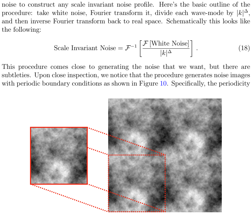
The machinery has three parts. First, a measurement: the Fourier-space covariance of a natural-image set is approximately diagonal and radial, $\Gamma_{kl}^{ij} \approx A^2/|k|^{2\Delta}\delta_{kl}^{ij}$ with $\Delta \approx 1.5$; this is the signature of scale-invariant noise, placing white noise at $\Delta=0$, pink noise at $\Delta=1$, and red noise at $\Delta=2$. Second, a construction: take white noise, divide each Fourier mode by $|k|^{\Delta}$, and invert; to avoid toroidal boundary artifacts, generate on a larger grid and crop the center, which preserves $\Delta$ by scale invariance. Third, a real-valued Fourier transform that rewrites the complex Fourier statistics as a real diagonal normal distribution, so the addition formula for diagonal normals applies to mixtures of cloud noise. That addition formula is the load-bearing identity: it preserves the power-law form under the noising schedule, which is why the jump trick and the constant-frequency signal-to-noise property hold.

What would settle it

Compute the Fourier-space covariance of a natural-image set and plot its radial profile on log-log axes: if the curve bends, the slope changes with frequency, or the off-diagonal correlations are not small, the constant-frequency signal-to-noise property fails.

Watch

Extended reading notes

Core claim

The paper's central claim is that a diffusion model can use scale-invariant 'cloud noise' instead of white noise without giving up the mathematical apparatus of diffusion. Because a natural-image set's covariance is approximately diagonal in Fourier space and follows the power law $\Gamma \approx A^2/|k|^{2\Delta}$, the noise can be generated by dividing white-noise Fourier modes by $|k|^{\Delta}$, and its statistics can be represented as a real diagonal normal distribution. Diagonal normal distributions are closed under the linear combinations used in noising, so the jump trick survives: $x_t = \sqrt{\bar\alpha_t}x_0 + \sqrt{1-\bar\alpha_t}\varepsilon_{0:t}$ with $\varepsilon$ a cloud-noise sample. The forward distribution then has covariance $\Gamma \approx A^2/|k|^{2\Delta}\delta$ at every timestep, meaning signal-to-noise is flat across frequencies and reverse denoising refines all frequencies simultaneously. From that property the paper derives three promised benefits: fewer timesteps, better high-frequency fidelity, and more effective conditioning on high-frequency content.

Load-bearing premise

The argument assumes that an image set's correlations in frequency space are independent across frequencies and follow a single power law across all scales—and the evidence offered is a single fit to one cleaned natural-image set.

Editorial extensions

If this is right

The jump trick carries over unchanged, so cloud diffusion can reuse standard diffusion training objectives and noising schedules.
Reverse sampling no longer defers high-frequency detail to the last timesteps, so textures and edges receive corrective feedback throughout the reverse process rather than only at the end.
Because signal-to-noise is flat in frequency, the model has a shorter path from noise to data, so fewer denoising steps may suffice for good images.
Prompts that specify high-frequency content, such as a small object or a face in a crowd, can steer generation at every timestep instead of only in the final stages.

Reading between the lines

Editorial extensions of the paper, not claims the author makes directly.

An extension the paper leaves implicit: if the scaling exponent $\Delta$ drifts with frequency or with dataset, a single cloud-noise profile cannot deliver the promised flat signal-to-noise, and a multi-exponent or spatially varying noise would be the natural repair.
Because the paper's distance argument is distributional, the same construction should carry over to audio and scientific-imaging datasets whose power-law spectra are often better characterized than natural images; there the 'closer noise' claim could be tested directly.
The decisive evidence is still ahead: the paper itself plans a companion training study, so the promised benefits should be read as predictions from the covariance identity rather than demonstrated results.

Share X Bluesky LinkedIn Reddit HN

Editorial analysis

A structured set of objections, weighed in public.

Desk editor's note, referee report, and a circularity audit.

Desk Editor's Note

read the letter

Here's the short version: the paper's core trick — replacing white noise with dataset-tuned power-law noise while preserving the diffusion jump trick — is genuinely new to me, and the closure calculation (Eq. 32) is clean and correct. But the advertised benefits (faster inference, better details, improved conditioning) are argued from intuition and analogy, not derived or measured. The Mahalanobis "closer" result is partly circular because the reference distribution is defined to have exactly the cloud-noise covariance, so the distance is baked in. None of this sinks the paper; it just means you should read it as a position piece, not a finished result.

What's actually good: the Gaussian closure property is shown carefully, and the real Fourier transform construction is described in enough detail to reproduce. The paper is honest about what it doesn't show, and it correctly identifies that if the noise covariance matches the data covariance in the Fourier-diagonal basis, the aggregate covariance of the noised distribution becomes time-independent (Eq. 37). That is a genuinely interesting property, and I don't know prior work that combines it with the jump trick. The acknowledgment of Falck et al. is also honest.

Where it gets soft: Eq. 37 is a statement about the forward process. It says nothing directly about the length of the reverse trajectory, the score estimation error, or the truncation error of a finite-step sampler. Shorter Mahalanobis distance between cloud noise and the dataset is not evidence of a shorter ODE/SDE path; the reference distribution in Eq. 43 is chosen to have the same covariance as the proposed noise, so the comparison is rigged in its favor. The high-frequency detail and conditioning arguments are plausible but remain at the level of spectral-autoregression and Where's Waldo thought experiments. The empirical support is a single power-law fit to a cleaned STL10 subset with masked modes and no error bars; if real datasets deviate from a pure diagonal power law, Eq. 37 is approximate.

These are proportionate objections. For a theory-and-motivation paper that explicitly defers experiments to Part 2, this is a legitimate contribution. The right referee will check the real Fourier transform construction and push for a direct link between the covariance closure and sampler efficiency.

Who should read it: people working on noise schedules, spectral methods in diffusion, or colored-noise alternatives to the standard Gaussian forward process. It deserves a serious referee, though the referee should treat it as an opening bid. I'd bring it to a reading group and cite it as related work if I were writing about spectral noise in diffusion.

Referee Report

4 major / 5 minor

Summary. The paper proposes replacing white noise in diffusion forward processes with "Cloud Noise," a power-law (1/|k|^{2\Delta}) Gaussian noise whose scaling exponent is fitted to the image set. It constructs a real-valued Fourier transform, shows that such scale-invariant noises close under linear combinations, derives a jump trick (Eq. 34), and argues that the resulting constant frequency-wise signal-to-noise ratio (Eq. 37) yields faster inference, better high-frequency detail, and improved conditional guidance. Empirical content is limited to a single power-law fit to a cleaned STL10 subset; all performance claims are deferred to a promised companion paper.

Significance. If the covariance-closure property (Eq. 37) and the associated benefits were validated, this would be a meaningful contribution: it would extend the standard diffusion jump trick to a broad class of 1/f^\alpha noises and potentially improve sample efficiency and high-frequency fidelity. The paper's formal construction of a real Fourier transform and the addition formula (Eq. 32) are clear and, under the stated idealizations, correct. However, the manuscript does not currently establish the advertised improvements: the distance argument is largely definitional, and the details and guidance arguments are heuristic. The empirical basis for the key assumption is thin. The paper is honest about deferring validation to Part 2, but that makes it more a position paper than a complete research article.

major comments (4)

[§4.1, Eq. (43) and Fig. 19] The reference distribution Q0 is defined to have covariance 1/|k|^{2\Delta}, exactly the cloud-noise covariance, so the comparison in Fig. 19 largely restates the covariance-matching assumption rather than independently measuring distance. Moreover, no bound or estimate links the Mahalanobis distances to the length of the probability-flow ODE/SDE trajectory, to the truncation error of a finite-step sampler, or to the number of required reverse steps; the "faster inference" conclusion is therefore not derived.
[§3.3, Eq. (37)] The frequency-independent SNR property holds only if the data covariance is exactly diagonal and power-law, approximately A^2/|k|^{2\Delta}, and if the cropped cloud-noise samples retain exactly that covariance. The only empirical support is a single linear fit to a cleaned, grayscale, 96x96 STL10 subset with the central cross masked (Fig. 9, Eq. 14), reported without error bars, dataset variation, or a test of the diagonal assumption; for real image sets, non-diagonal residues, scale-dependent Delta, or masking effects would break Eq. (37). This is load-bearing because all three promised benefits are traced back to Eq. (37).
[§3.2, Eqs. (31)-(34)] The cropping trick is justified by scale invariance, but cropping a finite periodic field introduces spectral leakage, so the cropped noise's covariance in its own Fourier basis is not exactly diagonal or exactly 1/|k|^{2\Delta}. Since Eq. (31) is the basis for the addition formula (32) and the jump trick (34), the closure is approximate at best; the manuscript should quantify the approximation or verify it empirically.
[§4.2 and §4.3] The "better details" and "improved conditional guidance" claims are argued by analogy and by Bayesian intuition, not derived from score-estimation error, conditioning information, or sampling bounds. Section 5 explicitly defers training and comparison to Part 2, so the manuscript's central value claims remain unverified. A standalone paper should either provide experimental evidence, derive a formal bound, or clearly label these claims as conjectures.

minor comments (5)

[General] There are several typographical errors, including "T able 1" and "and and use that" in Section 2.3; these should be corrected.
[References] Reference [Fal+25] is discussed in the Acknowledgments but never cited in the body; add a related-work discussion in Section 1 or Section 3.
[Fig. 9 / Eq. (14)] Report the fit statistics for the power-law estimate, including parameter uncertainties and a goodness-of-fit measure, and state explicitly how the mask affects the fitted Delta.
[§3.3, Eq. (37)] Equation (37) is written with an approximation sign, but the surrounding text often treats it as exact ("the covariance is the same at each time step"); use consistent language, for example "holds to the accuracy of Eq. (14)."
[§2.5] Cloud Noise is coined as a new term, but it is never given a precise formal definition as a probability measure; define it explicitly, including the effect of the cropping procedure, before using it in the noising equations.

Circularity Check

1 steps flagged · score 6.0 of 10

The quantified claim that Cloud Noise is closer to the image set is built into the Mahalanobis reference distribution; the closure property is genuine but does not by itself establish the advertised benefits.

self definitional [Section 4.1, Eq. (43) and Figure 19]
"We’ll work in Real Fourier Space, and take the reference eQ0 to be the idealized distribution with covariance eΣij kl = 1 |k|2∆ δij kl. ... The Mahalanobis distance is then dM (X, Y |Q0) = q (Xij − Yij)|k|2∆(X ij − Y ij) (43) ... The values from the figure quantify what we mean by Cloud Noise is closer to the image set."

The reference distribution Q0 is defined to have the same power-law covariance 1/|k|^(2Δ) that defines Cloud Noise (Eq. 31, Table 2), and the image-set covariance was already modeled as A^2/|k|^(2Δ) (Eq. 14). Weighting squared differences by the inverse of that covariance, |k|^(2Δ), makes any distribution in the same 1/|k|^(2Δ) family (the image model and Cloud Noise) have comparable, k-independent Mahalanobis distances, while white noise's flat spectrum receives large high-frequency penalties. The conclusion 'Cloud Noise is closer to the image set' is therefore not an independent measurement but a restatement of the choice of metric/reference; it is forced by construction.

full rationale

The paper's central algebraic result, the closure of scale-invariant normal distributions under the forward noising combination (Eq. 32), is a genuine self-contained derivation from the diagonal-normal addition formula (Eq. 24); it is not circular. Equation (37), the constancy of the noisy covariance, is likewise a mathematical consequence of choosing the noise covariance to match the assumed image covariance, so it is true by construction rather than an independent discovery. The principal circularity is in Section 4.1, where the Mahalanobis reference distribution is given exactly the Cloud Noise covariance profile, so the quantified 'closer' claim reduces to the definition of the metric. No load-bearing self-citation or imported uniqueness theorem appears; [Ran24] is only a code repository reference. The three advertised benefits (speed, detail, conditional guidance) are argued from the constant-SNR property by heuristic analogy rather than derived, and the paper explicitly defers the decisive comparison to Part 2. The score reflects one supporting pillar that reduces by construction plus a central derivation that is otherwise independent.

Assumptions & free parameters 3 free parameters · 6 assumptions · 1 invented entities

The central design rests on Delta fitted to one dataset, a diagonal-covariance approximation, and a Gaussian model of image statistics. The closure property is mathematically sound, but the practical benefits depend on additional assumptions that are not yet tested.

free parameters (3)

Delta (scaling parameter) = ~1.5
Fitted from log-log slope of the covariance of a cleaned STL10 subset (Section 2.4, Eq. 14). This is the central design knob of Cloud Noise.
A (amplitude) = unspecified
Amplitude of the power-law covariance; adjusted to unit variance after cropping (Section 2.5). Not load-bearing for the shape but used in noise generation.
Crop factor (linear dimension multiplier) = 3
Hand-chosen practical value: 3N x 3N noise cropped to N x N to reduce periodic boundary artifacts (Section 2.5).

assumptions (6)

domain assumption Natural images have power-law two-point statistics (approx. 1/f^(2Δ)).
Invoked throughout Section 2, based on prior literature (Ruderman et al.). The paper measures it on STL10, but assumes general applicability.
domain assumption The image-set covariance in Fourier space is approximately diagonal.
Eq. (12) states the diagonal approximation. Needed for the closure property and for the constant-SNR argument.
domain assumption The image distribution can be modeled as a multivariate normal with that covariance.
Section 2.5 models the image set this way; the paper acknowledges higher-order moments (kurtosis) exist but ignores them.
standard math Sums of independent normal distributions are normal, and rescaling preserves normality.
Eqs. (22)-(24) give the standard Gaussian addition formula; this is not in question.
standard math The Real Fourier Transform is real-linear and invertible.
Section 3.2 defines the transform and asserts invertibility; this is a construction based on the standard FFT.
ad hoc to paper Cropping the center of a larger scale-invariant noise field preserves the scaling parameter Delta.
Section 2.5 and Figure 11 assert this from scale invariance, without a rigorous finite-size proof.

invented entities (1)

Cloud Noise
purpose: A scale-invariant noise distribution with Delta near 1.5, intended to replace white noise in diffusion models so the noise matches the image set's low-order statistics.
The name is coined in this paper. It is a 1/f-style noise, not a new physical object, and no empirical validation is provided here; the promised follow-up would supply it.

how reviews work

0 comments

Cite this review

Pith. "Pith review of Cloud Diffusion Part 1: Theory and Motivation." pith.science (2026). https://pith.science/paper/VMS2IWWU

@misc{pith2026250705496,
  author       = {Pith},
  title        = {Pith review of: Cloud Diffusion Part 1: Theory and Motivation},
  year         = {2026},
  howpublished = {\url{https://pith.science/paper/VMS2IWWU}},
  note         = {Machine review of arXiv:2507.05496}
}

read the original abstract

Diffusion models for image generation function by progressively adding noise to an image set and training a model to separate out the signal from the noise. The noise profile used by these models is white noise -- that is, noise based on independent normal distributions at each point whose mean and variance is independent of the scale. By contrast, most natural image sets exhibit a type of scale invariance in their low-order statistical properties characterized by a power-law scaling. Consequently, natural images are closer (in a quantifiable sense) to a different probability distribution that emphasizes large scale correlations and de-emphasizes small scale correlations. These scale invariant noise profiles can be incorporated into diffusion models in place of white noise to form what we will call a ``Cloud Diffusion Model". We argue that these models can lead to faster inference, improved high-frequency details, and greater controllability. In a follow-up paper, we will build and train a Cloud Diffusion Model that uses scale invariance at a fundamental level and compare it to classic, white noise diffusion models.

Figures

Figures reproduced from arXiv: 2507.05496 by the authors.

**Figure 1.** Cloud Diffusion uses scale-invariant noise tuned to the statistical properties of the image set in place of white noise to improve the generative model. Visualized here is the forward diffusion process for white noise diffusion models (top row) and for Cloud Diffusion Models (bottom row). This work is adapted from a series of Jupyter Notebooks and associated code posted in a public GitHub repository [Ran24]. Much of… view at source ↗

**Figure 2.** The images are a cleaned subset of the STL10 dataset. A handful of images are selected at random from the image set, and two points from each image are selected at random. You are given the coordinates of the two points, and the value of just one. You are also told the image set is a cleaned subset of the STL10 dataset, with images containing vertical or horizontal bars on the edges (typical artifacts of cropping) r… view at source ↗

**Figure 3.** The pixel-wise mean (first row) and standard deviation (second row) of the image set. The first column has plot range [0,1], and the second column is enhanced with plot range from the minimum to the maximum values. The plots reveal that while there is some variation in the mean and standard deviation, they are both extremely uniform over all pixels. 6 [PITH_FULL_IMAGE:figures/full_fig_p006_3.png] view at source ↗

Figures from the paper (18 more)

**Figure 4.** Figure 4: Random samples from the image set shown alongside samples of white noise. Though the noise samples have a pixel-wise mean and standard deviation that is tuned to match that of the dataset, the noise samples capture very little information about the set and look nothing…

**Figure 5.** Figure 5: The Covariance Tensor of the image set plotted for four randomly selected points. The plots reveal that neighboring pixels are correlated, and the magnitude of the correlation falls off with radial distance. between neighboring pixels is highest between immediately adj…

**Figure 6.** Figure 6: Four random sample images from the dataset with plots of the real part, imaginary part, and absolute value of the Fourier transform of each sample. 10 [PITH_FULL_IMAGE:figures/full_fig_p010_6.png]

**Figure 7.** Figure 7: The Covariance Tensor of the image set in Fourier Space, plotted for four randomly chosen points. The first column shows Γ and the second C. The second two columns show Γ and C with the central cross region masked out. The plots reveal the expected relation between the…

**Figure 8.** Figure 8: Here we plot the diagonal component Γ ij diag of the covariance Γ ij jk in Fourier Space. With the central cross masked, the remaining functional dependence is close to radial and falls off with distance. distinctive, almost radial structure. If we ignore the central c…

**Figure 9.** Figure 9: The dependence of Γdiag as a function of |k| is plotted on a linear scale (left) and on a log-log scale (right). Points in the masked region of [PITH_FULL_IMAGE:figures/full_fig_p014_9.png]

**Figure 10.** Figure 10: The naive procedure for generating scale invariant noise produces noise with periodic boundary conditions. This is shown here by tiling the noise in a wallpaper pattern. Note that the image is continuous and smooth on the edges where the tiles meet. is toroidal, meani…

**Figure 11.** Figure 11: Producing periodic noise on a larger scale and cropping the center produces scale-invariant noise with aperiodic boundary conditions. deviation you want, but the scaling parameter ∆ will be unchanged. In practice we’ve found that tripling the linear dimensions of the …

**Figure 12.** Figure 12: Noise samples for White Noise, Pink Noise, Cloud Noise, and Red (Brownian) Noise. Increasing ∆ amplifies low-frequency modes and suppresses high-frequency modes. Cloud Noise has a scaling parameter tuned to the image dataset. 18 [PITH_FULL_IMAGE:figures/full_fig_p018…

**Figure 13.** Figure 13: The density fluctuations of the Cosmic Microwave Background radiation, measured by the Planck mission, exhibit a scale-invariant power spectrum similar to that of Cloud Noise [IPA; Geo]. The fundamental premise behind Cloud Diffusion is that the diffusion paradigm ca…

**Figure 14.** Figure 14: Here we visualize the diffusion noising procedure for white noise and for cloud noise. The noise schedule is shown in real space and in Fourier space where the absolute value is taken. to white noise in the forward diffusion process have been considered before (see fo…

**Figure 15.** Figure 15: For square tensors with even linear dimensions, the origin of the Fourier transform is necessarily off center, and the involution is not a simple rotation. Instead the left column and top row invert as depicted, while the bottom right square simply rotates 180◦ . C ij…

**Figure 16.** Figure 16: Under the involution, light red pixels map to light blue pixels. Solid red pixels are stationary, and they are real valued under the Fourier transform. The Real Fourier Transform takes the ordinary Fourier transform, then projects the light red squares into their real…

**Figure 17.** Figure 17: The reverse diffusion procedure for white noise and Cloud Noise. Removing white noise effectively exposes higher frequencies. By contrast, the signal to noise ratio increases uniformly across all frequencies as Cloud Noise is removed. is to distill higher and higher f…

**Figure 18.** Figure 18: The reverse diffusion process carves a path from the noise distributions to the generated image set. We expect that since Cloud Noise has scaling parameters that are tuned to dataset, the path should be shorter in some quantifiable sense. In fact, there is a natural m…

**Figure 19.** Figure 19: The Mahalanobis distances calculated between the various distributions as labeled. Note that Cloud Noise is clearly closer to the image set than white noise relative to this measure. 4.2 Better Details We argue here that Cloud Diffusion can yield better high frequency…

**Figure 20.** Figure 20: Images generated by diffusion models often exhibit a characteristic “airbrushed” or “ultra-processed” look, suggesting they poorly model the high frequency details of the image sets they are trained on. noise models, the noising procedure effectively hides high freque…

**Figure 21.** Figure 21 [PITH_FULL_IMAGE:figures/full_fig_p035_21.png]

Discussion (0). Continue with ORCID to comment.

Reference graph

Works this paper leans on

12 extracted references · 5 canonical work pages

[1]

Color and spatial structure in natural scenes

[BM87] Geoffrey J Burton and Ian R Moorhead. “Color and spatial structure in natural scenes”. In: Applied optics 26.1 (1987), pp. 157–170. [Fie87] David J Field. “Relations between the statistics of natural images and the response properties of cortical cells”. In: Journal of the Optical Society of America A 4.12 (1987), pp. 2379–2394. [TTC92] David J Tol...

1987
[9]

Cold diffusion: Inverting arbitrary image transforms without noise

arXiv: 2010 . 02502 [cs.LG]. url: https : / / arxiv.org/abs/2010.02502. [Ban+23] Arpit Bansal et al. “Cold diffusion: Inverting arbitrary image transforms without noise”. In: Advances in Neural Information Processing Systems 36 (2023), pp. 41259–41282. arXiv: 2208.09392 [cs.CV]. url: https: //arxiv.org/abs/2208.09392. [Cro+23] Florinel-Alin Croitoru et al...

arXiv 2023
[33]

Scale invariance and noise in natural im- ages

[ZW09] Daniel Zoran and Yair Weiss. “Scale invariance and noise in natural im- ages”. In: 2009 IEEE 12th International Conference on Computer Vision. 2009, pp. 2209–2216. doi: 10.1109/ICCV.2009.5459476. [Soh+15] Jascha Sohl-Dickstein et al. “Deep unsupervised learning using nonequi- librium thermodynamics”. In: International conference on machine learn- i...

work page arXiv 2018
[345]

Modelling the power spectra of natural images: statistics and information

36 [VH96] van A Van der Schaaf and JH van van Hateren. “Modelling the power spectra of natural images: statistics and information”. In: Vision research 36.17 (1996), pp. 2759–2770. [Han97] Martin Hanford. Where’s Waldo Now? Candlewick, Oct

work page 1996
[814]

Statistics of natural time-varying images

[DA95] Dawei W Dong and Joseph J Atick. “Statistics of natural time-varying images”. In: Network: computation in neural systems 6.3 (1995), p

work page 1995
[1997]

Origins of scaling in natural images

isbn: 0763603082. [Rud97] Daniel L Ruderman. “Origins of scaling in natural images”. In: Vision research 37.23 (1997), pp. 3385–3398. [Sri+03] Anuj Srivastava et al. “On advances in statistical modeling of natural im- ages”. In: Journal of mathematical imaging and vision 18 (2003), pp. 17–

work page 1997
[2020]

Diffusion models beat gans on image synthesis

arXiv: 2006.11239 [cs.LG]. url: https://arxiv. org/abs/2006.11239. [DN21] Prafulla Dhariwal and Alexander Nichol. “Diffusion models beat gans on image synthesis”. In: Advances in neural information processing systems 34 (2021), pp. 8780–8794. arXiv: 2105 . 05233 [cs.LG]. url: https : //arxiv.org/abs/2105.05233. [Son+21] Yang Song et al. Score-Based Genera...

arXiv 2021
[2021]

url: https: //arxiv.org/abs/2011.13456

arXiv: 2011.13456 [cs.LG]. url: https: //arxiv.org/abs/2011.13456. [HS22] Jonathan Ho and Tim Salimans. Classifier-Free Diffusion Guidance

arXiv 2011

Show all 12 references

[2022]

High-resolution image synthesis with latent diffu- sion models

arXiv: 2208 . 11970 [cs.LG]. url: https : / / arxiv . org / abs / 2208 . 11970. [Rom+22] Robin Rombach et al. “High-resolution image synthesis with latent diffu- sion models”. In: Proceedings of the IEEE/CVF conference on computer vision and pattern recognition. 2022, pp. 1068...

2022 arXiv
[2024]

[Ran24] Andrew Randono

url: https://sander.ai/2024/09/02/spectral-autoregression.html. [Ran24] Andrew Randono. Cloud Diffusion

2024
[2025]

url: https://arxiv.org/abs/ 2505.11278

arXiv: 2505.11278 [stat.ML]. url: https://arxiv.org/abs/ 2505.11278. [Geo] Damien P. George. Interactive visualization of the temperature fluctua- tions of the CMB observed by the Planck mission. url: http://thecmb. org. 38 [IPA] IPAC. Credit: ESA and the Planck Collaboration....

arXiv
[2209]

url: https://arxiv.org/abs/2209.02646

02646 [cs.AI]. url: https://arxiv.org/abs/2209.02646. [Die24] Sander Dieleman. Diffusion is spectral autoregression . Sept

arXiv

Pith tools

Reviewed August 6, 2026 · model on record in the stance chip above.

[1] [1]

Color and spatial structure in natural scenes

[BM87] Geoffrey J Burton and Ian R Moorhead. “Color and spatial structure in natural scenes”. In: Applied optics 26.1 (1987), pp. 157–170. [Fie87] David J Field. “Relations between the statistics of natural images and the response properties of cortical cells”. In: Journal of the Optical Society of America A 4.12 (1987), pp. 2379–2394. [TTC92] David J Tol...

1987

[2] [9]

Cold diffusion: Inverting arbitrary image transforms without noise

arXiv: 2010 . 02502 [cs.LG]. url: https : / / arxiv.org/abs/2010.02502. [Ban+23] Arpit Bansal et al. “Cold diffusion: Inverting arbitrary image transforms without noise”. In: Advances in Neural Information Processing Systems 36 (2023), pp. 41259–41282. arXiv: 2208.09392 [cs.CV]. url: https: //arxiv.org/abs/2208.09392. [Cro+23] Florinel-Alin Croitoru et al...

arXiv 2023

[3] [33]

Scale invariance and noise in natural im- ages

[ZW09] Daniel Zoran and Yair Weiss. “Scale invariance and noise in natural im- ages”. In: 2009 IEEE 12th International Conference on Computer Vision. 2009, pp. 2209–2216. doi: 10.1109/ICCV.2009.5459476. [Soh+15] Jascha Sohl-Dickstein et al. “Deep unsupervised learning using nonequi- librium thermodynamics”. In: International conference on machine learn- i...

work page arXiv 2018

[4] [345]

Modelling the power spectra of natural images: statistics and information

36 [VH96] van A Van der Schaaf and JH van van Hateren. “Modelling the power spectra of natural images: statistics and information”. In: Vision research 36.17 (1996), pp. 2759–2770. [Han97] Martin Hanford. Where’s Waldo Now? Candlewick, Oct

work page 1996

[5] [814]

Statistics of natural time-varying images

[DA95] Dawei W Dong and Joseph J Atick. “Statistics of natural time-varying images”. In: Network: computation in neural systems 6.3 (1995), p

work page 1995

[6] [1997]

Origins of scaling in natural images

isbn: 0763603082. [Rud97] Daniel L Ruderman. “Origins of scaling in natural images”. In: Vision research 37.23 (1997), pp. 3385–3398. [Sri+03] Anuj Srivastava et al. “On advances in statistical modeling of natural im- ages”. In: Journal of mathematical imaging and vision 18 (2003), pp. 17–

work page 1997

[7] [2020]

Diffusion models beat gans on image synthesis

arXiv: 2006.11239 [cs.LG]. url: https://arxiv. org/abs/2006.11239. [DN21] Prafulla Dhariwal and Alexander Nichol. “Diffusion models beat gans on image synthesis”. In: Advances in neural information processing systems 34 (2021), pp. 8780–8794. arXiv: 2105 . 05233 [cs.LG]. url: https : //arxiv.org/abs/2105.05233. [Son+21] Yang Song et al. Score-Based Genera...

arXiv 2021

[8] [2021]

url: https: //arxiv.org/abs/2011.13456

arXiv: 2011.13456 [cs.LG]. url: https: //arxiv.org/abs/2011.13456. [HS22] Jonathan Ho and Tim Salimans. Classifier-Free Diffusion Guidance

arXiv 2011